Lab 2: Variable Selection in R

In this lab, you will learn how

To perform forward and backward stepwise selection using different model selection criteria.
To perform best subset selection.
To fit a linear model by LASSO and to choose the tuning parameter by cross-validation.

In this lab, we will be using the following blood pressure dataset. This dataset contains measurements possibly related to blood pressure from 39 Peruvians who moved from rural high altitude areas to urban lower altitude areas. The dataset contains the following variables:

Y = systolic blood pressure
\(X_1\) = age
\(X_2\) = years in urban area
\(X_3\) = \(X_2/X_1\) = fraction of life in an urban area
\(X_4\) = weight in kg
\(X_5\) = height in mm
\(X_6\) = chin skinfold
\(X_7\) = forearm skinfold
\(X_8\) = calf skinfold
\(X_9\) = resting pulse rate

For linear regression, the leaps library contains the function regsubsets() that can be used for forward, backward and best subset selection. The function, regsubsets() has four main arguments:

formula - this states the largest possible regression model in question, that is, the the response and all the eligible predictors
data - the data.frame containing these variables
nbest - the number of best models to show for each set of \(k\) variable models
nvmax - maximum size of subsets to examine (default is 8)
method - forward, backward, or exhaustive (best)

Let’s begin with best subset selection:

peru.dat <- read.csv("Data/peru.csv",header=T)

write.csv(peru.dat,"Data/peru.csv")

library(leaps)

## Warning: package 'leaps' was built under R version 3.4.3

peru.best <- regsubsets(Systol ~ Age+Years+Weight+Height+Chin+Forearm+Calf+Pulse+UrbanFrac,data=peru.dat,nbest=2,nvmax=9,method="exhaustive")
peru.subsets <- summary(peru.best)
cbind(peru.subsets$outmat,"R2"=round(peru.subsets$rsq,4),"Adjusted R2"=round(peru.subsets$adjr2,4),"Cp"=round(peru.subsets$cp,4),"BIC"=round(peru.subsets$bic,4))

##          Age Years Weight Height Chin Forearm Calf Pulse UrbanFrac
## 1  ( 1 ) " " " "   "*"    " "    " "  " "     " "  " "   " "      
## 1  ( 2 ) " " " "   " "    " "    " "  " "     " "  " "   "*"      
## 2  ( 1 ) " " " "   "*"    " "    " "  " "     " "  " "   "*"      
## 2  ( 2 ) " " "*"   "*"    " "    " "  " "     " "  " "   " "      
## 3  ( 1 ) " " " "   "*"    " "    "*"  " "     " "  " "   "*"      
## 3  ( 2 ) " " "*"   "*"    " "    " "  " "     " "  " "   "*"      
## 4  ( 1 ) "*" "*"   "*"    " "    " "  " "     " "  " "   "*"      
## 4  ( 2 ) "*" "*"   " "    "*"    " "  " "     " "  " "   "*"      
## 5  ( 1 ) "*" "*"   "*"    " "    "*"  " "     " "  " "   "*"      
## 5  ( 2 ) "*" "*"   "*"    " "    " "  "*"     " "  " "   "*"      
## 6  ( 1 ) "*" "*"   "*"    " "    "*"  "*"     " "  " "   "*"      
## 6  ( 2 ) "*" "*"   "*"    " "    "*"  " "     "*"  " "   "*"      
## 7  ( 1 ) "*" "*"   "*"    "*"    "*"  "*"     " "  " "   "*"      
## 7  ( 2 ) "*" "*"   "*"    " "    "*"  "*"     " "  "*"   "*"      
## 8  ( 1 ) "*" "*"   "*"    "*"    "*"  "*"     " "  "*"   "*"      
## 8  ( 2 ) "*" "*"   "*"    "*"    "*"  "*"     "*"  " "   "*"      
## 9  ( 1 ) "*" "*"   "*"    "*"    "*"  "*"     "*"  "*"   "*"      
##          R2       Adjusted R2 Cp        BIC       
## 1  ( 1 ) "0.2718" "0.2521"    "28.4846" "-5.044"  
## 1  ( 2 ) "0.0763" "0.0513"    "45.5344" "4.2336"  
## 2  ( 1 ) "0.4731" "0.4438"    "12.9359" "-13.9989"
## 2  ( 2 ) "0.4208" "0.3886"    "17.4982" "-10.306" 
## 3  ( 1 ) "0.5033" "0.4608"    "12.3013" "-12.6388"
## 3  ( 2 ) "0.4905" "0.4468"    "13.4197" "-11.6444"
## 4  ( 1 ) "0.5974" "0.55"      "6.1018"  "-17.1626"
## 4  ( 2 ) "0.5252" "0.4694"    "12.3932" "-10.7328"
## 5  ( 1 ) "0.6386" "0.5839"    "4.5047"  "-17.7155"
## 5  ( 2 ) "0.6314" "0.5755"    "5.1386"  "-16.9386"
## 6  ( 1 ) "0.6488" "0.583"     "5.6167"  "-15.1671"
## 6  ( 2 ) "0.6487" "0.5828"    "5.6295"  "-15.1506"
## 7  ( 1 ) "0.6607" "0.584"     "6.5853"  "-12.8399"
## 7  ( 2 ) "0.6553" "0.5775"    "7.0513"  "-12.2303"
## 8  ( 1 ) "0.6664" "0.5774"    "8.0872"  "-9.8385" 
## 8  ( 2 ) "0.6622" "0.5721"    "8.4518"  "-9.3528" 
## 9  ( 1 ) "0.6674" "0.5641"    "10"      "-6.2921"

The summary function provides access to the model statistics such as \(R^2\), adjusted-\(R^2\), \(C_p\), and \(BIC\) as well as an object called outmat that contains the list of variables included in each model returned.

For forward stepwise selection, we just change the method to forward.

peru.best <- regsubsets(Systol ~ Age+Years+Weight+Height+Chin+Forearm+Calf+Pulse+UrbanFrac,data=peru.dat,nvmax=9,method="forward")
peru.subsets <- summary(peru.best)
cbind(peru.subsets$outmat,"R2"=round(peru.subsets$rsq,4),"Adjusted R2"=round(peru.subsets$adjr2,4),"Cp"=round(peru.subsets$cp,4),"BIC"=round(peru.subsets$bic,4))

##          Age Years Weight Height Chin Forearm Calf Pulse UrbanFrac
## 1  ( 1 ) " " " "   "*"    " "    " "  " "     " "  " "   " "      
## 2  ( 1 ) " " " "   "*"    " "    " "  " "     " "  " "   "*"      
## 3  ( 1 ) " " " "   "*"    " "    "*"  " "     " "  " "   "*"      
## 4  ( 1 ) "*" " "   "*"    " "    "*"  " "     " "  " "   "*"      
## 5  ( 1 ) "*" "*"   "*"    " "    "*"  " "     " "  " "   "*"      
## 6  ( 1 ) "*" "*"   "*"    " "    "*"  "*"     " "  " "   "*"      
## 7  ( 1 ) "*" "*"   "*"    "*"    "*"  "*"     " "  " "   "*"      
## 8  ( 1 ) "*" "*"   "*"    "*"    "*"  "*"     " "  "*"   "*"      
## 9  ( 1 ) "*" "*"   "*"    "*"    "*"  "*"     "*"  "*"   "*"      
##          R2       Adjusted R2 Cp        BIC       
## 1  ( 1 ) "0.2718" "0.2521"    "28.4846" "-5.044"  
## 2  ( 1 ) "0.4731" "0.4438"    "12.9359" "-13.9989"
## 3  ( 1 ) "0.5033" "0.4608"    "12.3013" "-12.6388"
## 4  ( 1 ) "0.5236" "0.4676"    "12.5317" "-10.6026"
## 5  ( 1 ) "0.6386" "0.5839"    "4.5047"  "-17.7155"
## 6  ( 1 ) "0.6488" "0.583"     "5.6167"  "-15.1671"
## 7  ( 1 ) "0.6607" "0.584"     "6.5853"  "-12.8399"
## 8  ( 1 ) "0.6664" "0.5774"    "8.0872"  "-9.8385" 
## 9  ( 1 ) "0.6674" "0.5641"    "10"      "-6.2921"

Similarly, for backward stepwise selection, change the method to backward.

peru.best <- regsubsets(Systol ~ Age+Years+Weight+Height+Chin+Forearm+Calf+Pulse+UrbanFrac,data=peru.dat,nvmax=9,method="backward")
peru.subsets <- summary(peru.best)
cbind(peru.subsets$outmat,"R2"=round(peru.subsets$rsq,4),"Adjusted R2"=round(peru.subsets$adjr2,4),"Cp"=round(peru.subsets$cp,4),"BIC"=round(peru.subsets$bic,4))

##          Age Years Weight Height Chin Forearm Calf Pulse UrbanFrac
## 1  ( 1 ) " " " "   "*"    " "    " "  " "     " "  " "   " "      
## 2  ( 1 ) " " " "   "*"    " "    " "  " "     " "  " "   "*"      
## 3  ( 1 ) " " "*"   "*"    " "    " "  " "     " "  " "   "*"      
## 4  ( 1 ) "*" "*"   "*"    " "    " "  " "     " "  " "   "*"      
## 5  ( 1 ) "*" "*"   "*"    " "    "*"  " "     " "  " "   "*"      
## 6  ( 1 ) "*" "*"   "*"    " "    "*"  "*"     " "  " "   "*"      
## 7  ( 1 ) "*" "*"   "*"    "*"    "*"  "*"     " "  " "   "*"      
## 8  ( 1 ) "*" "*"   "*"    "*"    "*"  "*"     " "  "*"   "*"      
## 9  ( 1 ) "*" "*"   "*"    "*"    "*"  "*"     "*"  "*"   "*"      
##          R2       Adjusted R2 Cp        BIC       
## 1  ( 1 ) "0.2718" "0.2521"    "28.4846" "-5.044"  
## 2  ( 1 ) "0.4731" "0.4438"    "12.9359" "-13.9989"
## 3  ( 1 ) "0.4905" "0.4468"    "13.4197" "-11.6444"
## 4  ( 1 ) "0.5974" "0.55"      "6.1018"  "-17.1626"
## 5  ( 1 ) "0.6386" "0.5839"    "4.5047"  "-17.7155"
## 6  ( 1 ) "0.6488" "0.583"     "5.6167"  "-15.1671"
## 7  ( 1 ) "0.6607" "0.584"     "6.5853"  "-12.8399"
## 8  ( 1 ) "0.6664" "0.5774"    "8.0872"  "-9.8385" 
## 9  ( 1 ) "0.6674" "0.5641"    "10"      "-6.2921"

Notice, that in this example, the sequence of models is not the same for forward and backward stepwise selection.

For the lasso, we will need the function glmnet() in the glmnet package. To choose the tuning parameter by cross-validation, we can use the cv.glmnet() function. To perform the LASS, we set the alpha parameter to 1. In the cv.glmnet function, the nfolds argument determines the number of the cross-validation groups. If it is set to the total number of observations then it performs leave one out cross-validation. The predict function with type=“coefficient” can be used to extract the LASSO parameter estimates for a given choice of the tuning parameter denoted by s in the predict function.

set.seed(750)
library(glmnet)

## Warning: package 'glmnet' was built under R version 3.4.3

## Loading required package: Matrix

## Loading required package: foreach

## Warning: package 'foreach' was built under R version 3.4.3

## Loaded glmnet 2.0-13

cv.out <- cv.glmnet(as.matrix(peru.dat[,-c(9,10)]),peru.dat$Systol,alpha=1,nfolds=10)
plot(cv.out)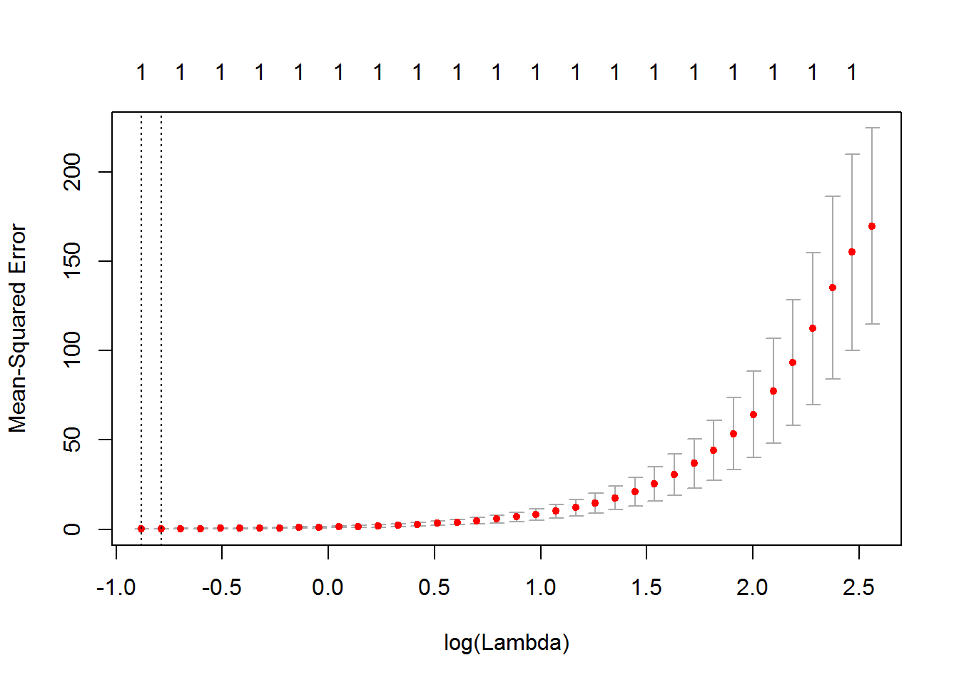

best.lam <- cv.out$lambda.min
best.lam

## [1] 0.4140212

peru.lasso <- glmnet(as.matrix(peru.dat[,-c(9,10)]),peru.dat$Systol,alpha=1)
predict(peru.lasso,type="coefficients",s=best.lam)

## 16 x 1 sparse Matrix of class "dgCMatrix"
##                     1
## (Intercept) 4.0761945
## X.5         .        
## X.4         .        
## X.3         .        
## X.2         .        
## X.1         .        
## X           .        
## Age         .        
## Years       .        
## Chin        .        
## Forearm     .        
## Calf        .        
## Pulse       .        
## Systol      0.9680073
## Diastol     .        
## UrbanFrac   .

Looking at the plot it would have been reasonable to also choose \(\lambda=e^{0.5}=1.648721\). This would result in the following LASSO fit.

predict(peru.lasso,type="coefficients",s=2.225541)

## 16 x 1 sparse Matrix of class "dgCMatrix"
##                      1
## (Intercept) 21.9112906
## X.5          .        
## X.4          .        
## X.3          .        
## X.2          .        
## X.1          .        
## X            .        
## Age          .        
## Years        .        
## Chin         .        
## Forearm      .        
## Calf         .        
## Pulse        .        
## Systol       0.8280257
## Diastol      .        
## UrbanFrac    .