Chapter 6 Data Summarization
In this section, we will learn the basics of exploratory data analysis in R. We will learn how to summarize one categorical variable, a character vector in R (or a factor, see Chapter 7), one quantitative variable, a numeric vector in R, and summaries of bivariate data. We will cover both numeric and the basics of graphical summaries. In Chapter 10, we will come back to plotting in more detail to see how to customize the plots (e.g. legends, axis labels, titles, etc.). For plotting, we will see both the base R plotting functions and plotting functions from ggplot2.
Throughout this chapter, we will use data from the HERS clinical trial for our examples. The Heart and Estrogen/progestin Replacement Study (HERS) trial was a randomized, blinded, placebo-controlled secondary prevention trial of estrogen plus progestin for secondary prevention of coronary heart disease (CHD) in postmenopausal women. For more information see the American College of Cardiology.
Warning: package 'readxl' was built under R version 4.3.2# A tibble: 6 × 37
HT age raceth nonwhite smoking drinkany exercise physact globrat poorfair
<chr> <dbl> <chr> <chr> <chr> <chr> <chr> <chr> <chr> <chr>
1 plac… 70 Afric… yes no no no much m… good no
2 plac… 62 Afric… yes no no no much l… good no
3 horm… 69 White no no no no about … good no
4 plac… 64 White no yes yes no much l… good no
5 plac… 65 White no no no no somewh… good no
6 horm… 68 Afric… yes no yes no about … good no
# ℹ 27 more variables: medcond <dbl>, htnmeds <chr>, statins <chr>,
# diabetes <chr>, dmpills <chr>, insulin <chr>, weight <dbl>, BMI <dbl>,
# waist <dbl>, WHR <dbl>, glucose <dbl>, weight1 <dbl>, BMI1 <dbl>,
# waist1 <dbl>, WHR1 <dbl>, glucose1 <dbl>, tchol <dbl>, LDL <dbl>,
# HDL <dbl>, TG <dbl>, tchol1 <dbl>, LDL1 <dbl>, HDL1 <dbl>, TG1 <dbl>,
# SBP <dbl>, DBP <dbl>, age10 <dbl>We will also make use of the Youth Tobacco Survey dataset,
# A tibble: 6 × 31
   YEAR LocationAbbr LocationDesc TopicType     TopicDesc MeasureDesc DataSource
  <dbl> <chr>        <chr>        <chr>         <chr>     <chr>       <chr>
1  2015 AZ           Arizona      Tobacco Use … Cessatio… Percent of… YTS
2  2015 AZ           Arizona      Tobacco Use … Cessatio… Percent of… YTS
3  2015 AZ           Arizona      Tobacco Use … Cessatio… Percent of… YTS
4  2015 AZ           Arizona      Tobacco Use … Cessatio… Quit Attem… YTS
5  2015 AZ           Arizona      Tobacco Use … Cessatio… Quit Attem… YTS
6  2015 AZ           Arizona      Tobacco Use … Cessatio… Quit Attem… YTS
# ℹ 24 more variables: Response <chr>, Data_Value_Unit <chr>,
#   Data_Value_Type <chr>, Data_Value <dbl>, Data_Value_Footnote_Symbol <chr>,
#   Data_Value_Footnote <chr>, Data_Value_Std_Err <dbl>,
#   Low_Confidence_Limit <dbl>, High_Confidence_Limit <dbl>, Sample_Size <dbl>,
#   Gender <chr>, Race <chr>, Age <chr>, Education <chr>, GeoLocation <chr>,
#   TopicTypeId <chr>, TopicId <chr>, MeasureId <chr>, StratificationID1 <chr>,
#   StratificationID2 <chr>, StratificationID3 <chr>, …
and the TB incidence dataset.
# A tibble: 6 × 19
TB incidence, all fo…¹ `1990` `1991` `1992` `1993` `1994` `1995` `1996` `1997`
<chr> <dbl> <dbl> <dbl> <dbl> <dbl> <dbl> <dbl> <dbl>
1 Afghanistan 168 168 168 168 168 168 168 168
2 Albania 25 24 25 26 26 27 27 28
3 Algeria 38 38 39 40 41 42 43 44
4 American Samoa 21 7 2 9 9 11 0 12
5 Andorra 36 34 32 30 29 27 26 26
6 Angola 205 209 214 218 222 226 231 236
# ℹ abbreviated name:
# ¹`TB incidence, all forms (per 100 000 population per year)`
# ℹ 10 more variables: `1998` <dbl>, `1999` <dbl>, `2000` <dbl>, `2001` <dbl>,
# `2002` <dbl>, `2003` <dbl>, `2004` <dbl>, `2005` <dbl>, `2006` <dbl>,
# `2007` <dbl>The first column of the TB incidence dataset should be renamed to “country”
[1] "TB incidence, all forms (per 100 000 population per year)"tb = tb %>% rename(country = "TB incidence, all forms (per 100 000 population per year)")
colnames(tb)[1][1] "country"6.1 One Quantitative Variable
6.1.1 Numeric Summaries
R has all of the standard numeric summary functions in base R including
mean(x): find the mean of a numeric vectorx.sd(x): find the standard deviation of a numeric vectorx.median(x): finds the median of a numeric vectorx.quantile(x): finds the sample quantiles of the numeric vectorx. Default is min, Q1, M, Q3, and max. Can find other quantiles by using theprobsargument.range(x): finds the range of the numeric vectorx. Displaysc(min(x), max(x)).sum(x): find the sum of the elements of the numeric vectorx.
All of these functions have an na.rm argument for missing data (discussed later).
R also has many mathematical functions that are useful for transformations (e.g. in regression modeling).
log- log (base e) transformationlog2- log base 2 transformationlog10- log base 10 transformationsqrt- square root transformation
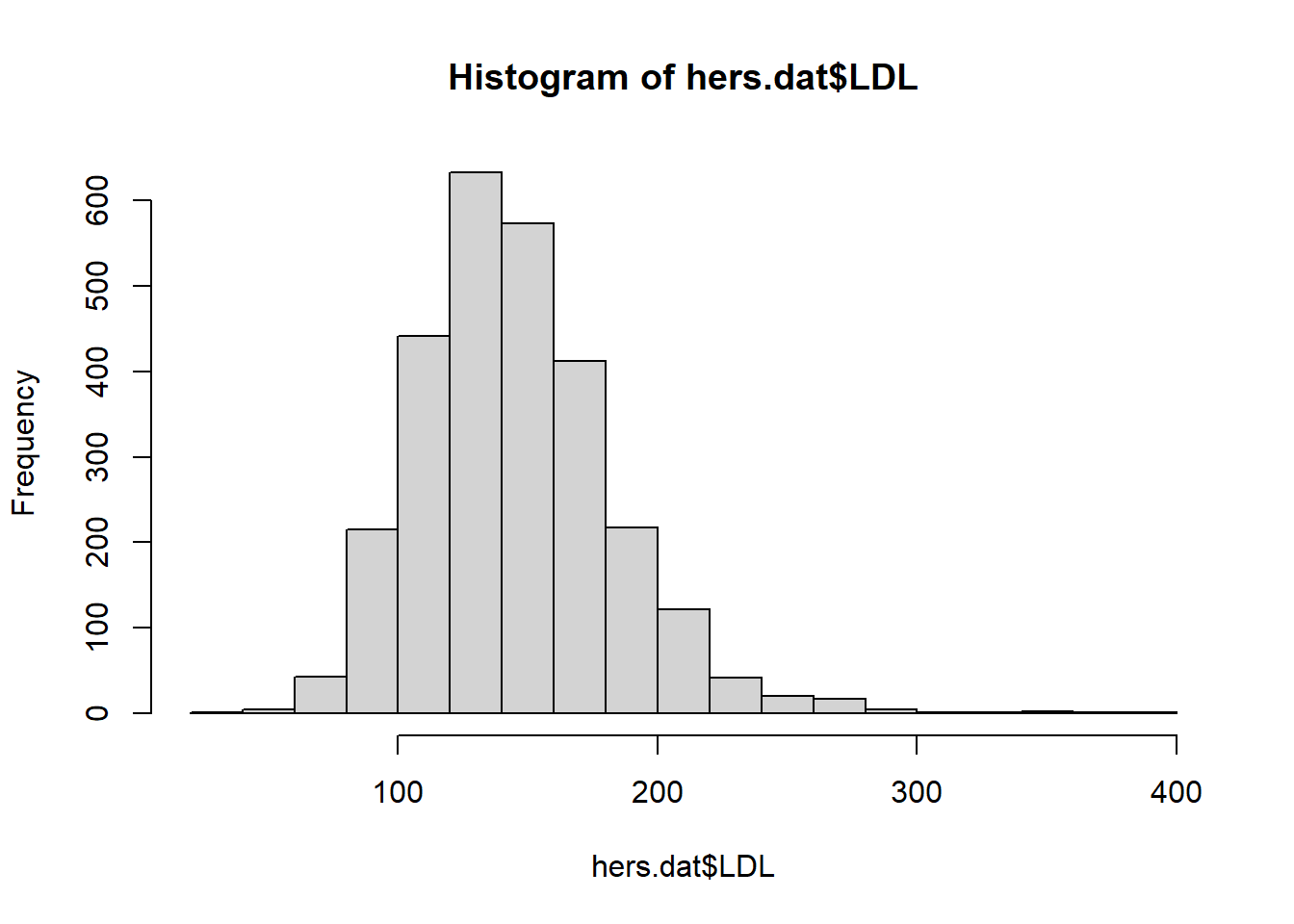
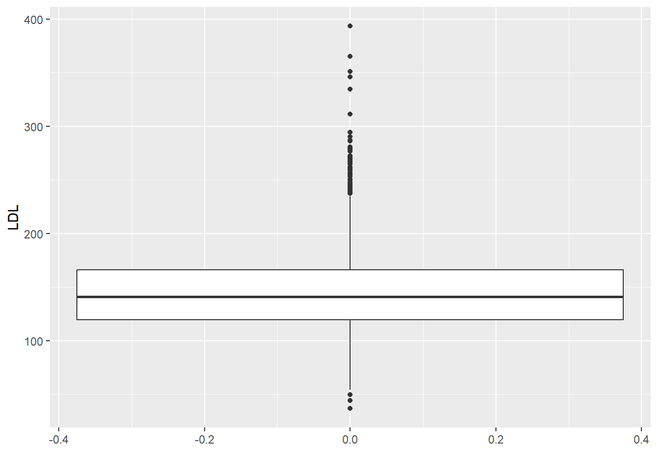
Let’s explore some of these numeric summaries using the HERS clinical trial data. Let’s numerically describe the distribution of LDL cholesterol levels. There are missing values in the LDL variable (patient’s LDL was not recorded for all patients). Missing data in R is recorded as NA. Calculations with NA results in an NA.
[1] NATo find summary statistics for the non-missing data, we can specify na.rm = TRUE which tells the R functions to exclude the NA values.
[1] 145.0385[1] 141[1] 37.80322 0% 25% 50% 75% 100%
36.8 119.6 141.0 166.0 393.4 60%
150.4 Sometimes you will have multiple columns or rows of a data.frame/matrix that you want to summarize. We can apply each of these functions to each of the columns/rows individually, but this can become tedious if you have many of them. In this case, there are fast functions built to work on all columns/rows. Note all columns/rows must be numeric.
rowMeans(x): finds the mean of each row ofxcolMeans(x): finds the mean of each column ofxrowSums(x): finds the sum of each row ofxcolSums(x): finds the sum of each column ofxsummary(x): for data.frames, display the quantile information and number of NAs
Additional packages such as matrixStats contain other row* and col* functions such as rowSds and colQuantiles.
For example, in the TB incidence dataset contains the TB incidence rate per year for the years 1990-2007 (some are missing) for a given country in each row. So if we wanted to calculate the average TB incidence rate over the years 1990-1999 for each country, we could used rowMeans, or we could find the average TB incidence rate per year over all these countries by using colMeans.
avgs = select(tb, starts_with("1")) # Select year columns 1990-1999
colMeans(avgs, na.rm = TRUE) #Average TB incidence per year
1990 1991 1992 1993 1994 1995 1996 1997
105.5797 107.6715 108.3140 110.3188 111.9662 114.1981 115.3527 118.8792
1998 1999
121.5169 125.0435 tb$before_2000_avg = rowMeans(avgs, na.rm = TRUE) # Average TB incidence from 1990-1999 for each country
head(tb[, c("country", "before_2000_avg")])# A tibble: 6 × 2
country before_2000_avg
<chr> <dbl>
1 Afghanistan 168
2 Albania 26.3
3 Algeria 41.8
4 American Samoa 8.5
5 Andorra 28.8
6 Angola 225. The summary function can give you a rough snapshot of each column, but in practice we would generally use mean, min, max, and quantile when needed.
country 1990 1991 1992
Length:208 Min. : 0.0 Min. : 4.0 Min. : 2.0
Class :character 1st Qu.: 27.5 1st Qu.: 27.0 1st Qu.: 27.0
Mode :character Median : 60.0 Median : 58.0 Median : 56.0
Mean :105.6 Mean :107.7 Mean :108.3
3rd Qu.:165.0 3rd Qu.:171.0 3rd Qu.:171.5
Max. :585.0 Max. :594.0 Max. :606.0
NA's :1 NA's :1 NA's :1
1993 1994 1995 1996 1997
Min. : 4.0 Min. : 0 Min. : 3.0 Min. : 0.0 Min. : 0.0
1st Qu.: 27.5 1st Qu.: 26 1st Qu.: 26.5 1st Qu.: 25.5 1st Qu.: 24.5
Median : 56.0 Median : 57 Median : 58.0 Median : 60.0 Median : 64.0
Mean :110.3 Mean :112 Mean :114.2 Mean :115.4 Mean :118.9
3rd Qu.:171.0 3rd Qu.:174 3rd Qu.:177.5 3rd Qu.:179.0 3rd Qu.:181.0
Max. :618.0 Max. :630 Max. :642.0 Max. :655.0 Max. :668.0
NA's :1 NA's :1 NA's :1 NA's :1 NA's :1
1998 1999 2000 2001
Min. : 0.0 Min. : 0.0 Min. : 0.0 Min. : 0.0
1st Qu.: 23.5 1st Qu.: 22.5 1st Qu.: 21.5 1st Qu.: 19.0
Median : 63.0 Median : 66.0 Median : 60.0 Median : 59.0
Mean :121.5 Mean :125.0 Mean :127.8 Mean :130.7
3rd Qu.:188.5 3rd Qu.:192.5 3rd Qu.:191.0 3rd Qu.:189.5
Max. :681.0 Max. :695.0 Max. :801.0 Max. :916.0
NA's :1 NA's :1 NA's :1 NA's :1
2002 2003 2004 2005
Min. : 3.0 Min. : 0.0 Min. : 0 Min. : 0.00
1st Qu.: 20.5 1st Qu.: 17.5 1st Qu.: 18 1st Qu.: 16.75
Median : 60.0 Median : 56.0 Median : 56 Median : 53.50
Mean :136.2 Mean : 136.2 Mean : 137 Mean : 135.67
3rd Qu.:195.5 3rd Qu.: 189.0 3rd Qu.: 184 3rd Qu.: 183.75
Max. :994.0 Max. :1075.0 Max. :1127 Max. :1141.00
NA's :1 NA's :1 NA's :1
2006 2007 before_2000_avg
Min. : 0.00 Min. : 0.0 Min. : 3.50
1st Qu.: 16.75 1st Qu.: 15.5 1st Qu.: 26.45
Median : 55.50 Median : 53.0 Median : 61.20
Mean : 134.61 Mean : 133.4 Mean :113.88
3rd Qu.: 185.00 3rd Qu.: 186.5 3rd Qu.:175.20
Max. :1169.00 Max. :1198.0 Max. :637.10
NA's :1 NA's :1 You can apply more general functions to the rows or columns of a matrix or data frame, beyond the mean and sum.
apply(X, MARGIN, FUN, ...)
- X: an array, including a matrix
- MARGIN: a vector giving the subscripts which the function will be applied over. E.g., for a matrix 1 indicates rows, 2 indicates columns, c(1,2) indicates rows and columns. When X has named dimnames, it can be a character vector selecting dimension names.
- FUN: the function to be applied: see ‘Details’
- …: optional arguments to FUN
    1990     1991     1992     1993     1994     1995     1996     1997
105.5797 107.6715 108.3140 110.3188 111.9662 114.1981 115.3527 118.8792
    1998     1999
121.5169 125.0435 [1] 168.0 26.3 41.8 8.5 28.8 224.6 1990 1991 1992 1993 1994 1995 1996 1997
110.6440 112.7687 114.4853 116.6744 120.0931 122.7119 126.1800 131.0858
1998 1999
137.3754 146.0755 1990 1991 1992 1993 1994 1995 1996 1997 1998 1999
585 594 606 618 630 642 655 668 681 695 There are other functions in the apply family such as
tapply(): grouping applylapply(): list apply (later)sapply(): simple apply (later)- Other less used ones
See more details here. These are commonly used, but we will discuss how to do all these using dplyr.
The dplyr function summarize allows you to make a tibble containing your requested summary statistics. The format is new = SUMMARY, where new is the variable name for the output statistic. If you do not provide a new name, then the output will be messy. Let’s find the average and median TB incidence rates for the years 2006 and 2007. (Note the use of backticks ``` to access the column names since they are numbers.)
tb %>%
  summarize(mean_2006 = mean(`2006`, na.rm = TRUE),
            median_2006 = median(`2006`, na.rm = TRUE),
            mean_2007 = mean(`2007`, na.rm = TRUE),
            median(`2007`, na.rm = TRUE))
# A tibble: 1 × 4
mean_2006 median_2006 mean_2007 `median(\`2007\`, na.rm = TRUE)`
<dbl> <dbl> <dbl> <dbl>
1 135. 55.5 133. 53dplyr also has a summarize_all function to apply a function to all columns like colMeans and colSums. For example, to find the average TB incidence rate for all years from 1990-199:
#summarize_all(DATASET, FUNCTION, OTHER_FUNCTION_ARGUMENTS) #how to use
summarize_all(avgs, mean, na.rm = TRUE)
# A tibble: 1 × 10
`1990` `1991` `1992` `1993` `1994` `1995` `1996` `1997` `1998` `1999`
<dbl> <dbl> <dbl> <dbl> <dbl> <dbl> <dbl> <dbl> <dbl> <dbl>
1 106. 108. 108. 110. 112. 114. 115. 119. 122. 125.6.1.2 Graphical Summaries
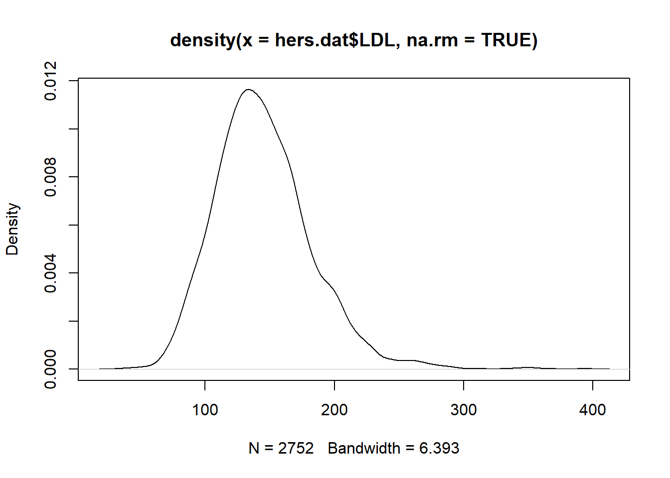
For one quantitative variable, we can summarize the data graphically using a
- histogram
- density plot
- boxplot
For base R plotting functions, we have
hist(x): makes a histogram from a numeric vectorxplot(density(x)): makes a density plot from a numeric vectorx(think a smoothed histogram)boxplot(x): makes a boxplot from the numeric vectorx

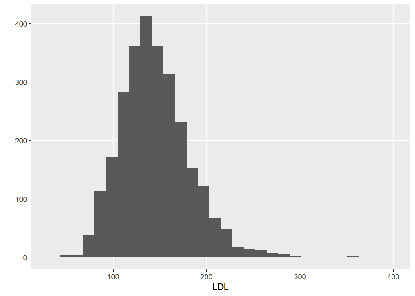
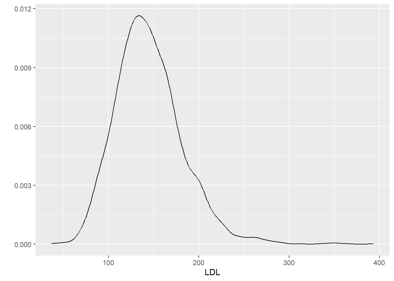
When using the ggplot2 package, we will focus on qplot (quick plot) for now. Later we will see how to use the more general ggplot function with layers. qplot has a few key inputs
x,y: the x and y variables to be plotteddata: name of the R data.frame that contains the variablesgeom: type of plot to makehistogram: to make a histogramdensity: to make a density plotboxplot: to make a boxplot
6.2 One Categorical Variable
6.2.1 Numeric Summaries
For a single categorical variable, we are interested in counts and proportions within each category. To find the counts, we can use the base R function table or with dplyr we can use the count.
Let’s examine the physact variable in the HERS dataset. unique(x) will return the unique elements of x, so we can see what the different categories of physical activity are.
[1] "much more active"     "much less active"     "about as active"
[4] "somewhat less active" "somewhat more active"
length will tell you the length of a vector. Combined with unique, it can tell you the number of unique elements. Using length with unique on the physact variable, we find that there are 5 levels.
[1] 5To count how many observations fall into each physical activity category, we can use table or count to construct a frequency table.
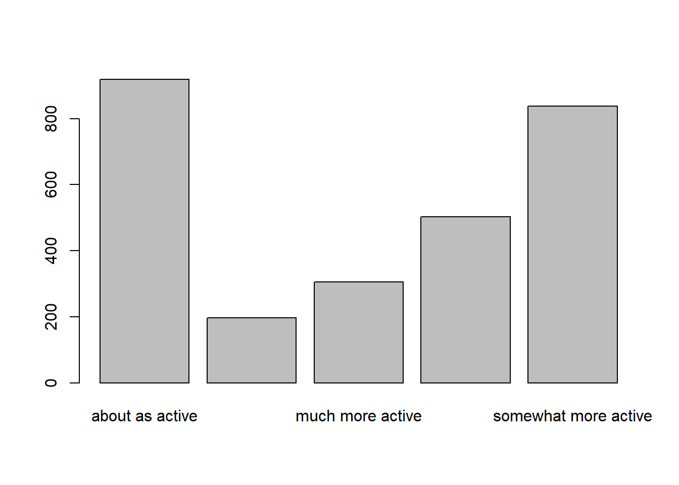
     about as active     much less active     much more active
                 919                  197                  306
somewhat less active somewhat more active
503 838 # A tibble: 5 × 2
physact n
<chr> <int>
1 about as active 919
2 much less active 197
3 much more active 306
4 somewhat less active 503
5 somewhat more active 838You may notice that the order of the categories is strange. We will learn how to fix this using factors in Chapter 7 by setting the levels in the desired order. Right now, R is using its default choice of alphanumeric order.
To find proportions/percentages, we can use prop.table. Notice that you need to apply prop.table to a table object.
     about as active     much less active     much more active
          0.33260948           0.07129931           0.11074919
somewhat less active somewhat more active
0.18204850 0.30329352 # A tibble: 5 × 3
physact n prop
<chr> <int> <dbl>
1 about as active 919 0.333
2 much less active 197 0.0713
3 much more active 306 0.111
4 somewhat less active 503 0.182
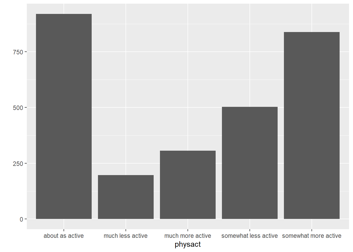
5 somewhat more active 838 0.303 6.2.2 Graphical Summaries
For one categorical variable, we graphically summarize it with a
- barplot
- pie chart
Base R has the functions barplot and pie to make these.
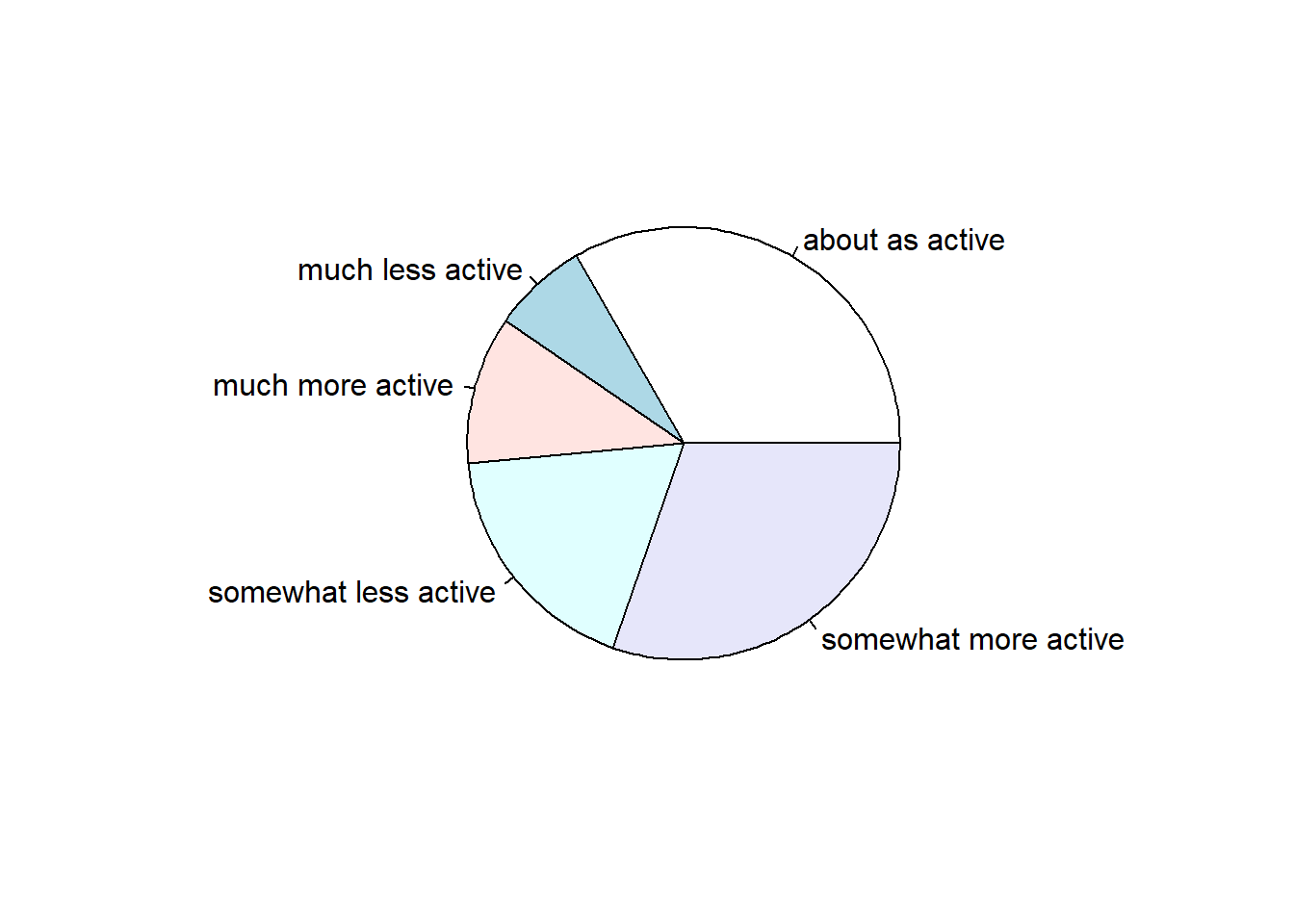
We can also make these using qplot. We use the bar geom for a barplot. A pie chart is slightly more complicated and will require the ggplot function. I will show you a pie chart here, but we will not cover ggplot until Chapter 10.
physact_cnt = hers.dat %>%
  count(physact) %>%
  mutate(prop = n / sum(n))
ggplot(physact_cnt, aes(x = "", y = prop, fill = physact)) +
  geom_bar(stat = "identity", width = 1)+
  coord_polar("y", start = 0)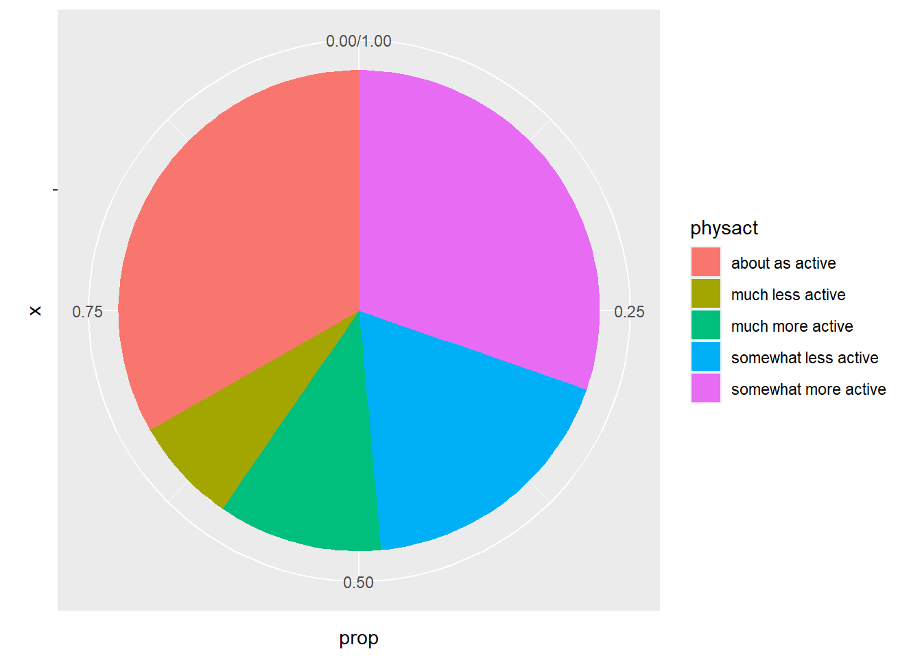
6.3 Case CC
When summarizing associations between two categorical variables, we are usually interested in contingency tables containing counts, overall proportions, row proportions, and/or column proportions. These can readily be made in R by using table and prop.table.
Let’s examine the association between smoking and physical activity. To see a contingency table of counts use table(x, y) where x and y are the two categorical variables.
                      smoking
physact                 no yes
  about as active      804 115
  much less active     155  42
  much more active     268  38
  somewhat less active 418  85
  somewhat more active 758  80
To find overall (AND) proportions, we pass this frequency table into prop.table.
                      smoking
physact                        no        yes
  about as active      0.29098806 0.04162143
  much less active     0.05609844 0.01520087
  much more active     0.09699602 0.01375317
  somewhat less active 0.15128484 0.03076366
  somewhat more active 0.27433949 0.02895404
We can see that the proportion that are both non-smokers and about as active is 0.29098806.
To find the conditional column percentages (in this case probability of being in a physical activity group, given smoking status), we would use prop.table with margin = 2.
                      smoking
physact                       no       yes
  about as active      0.3345818 0.3194444
  much less active     0.0645027 0.1166667
  much more active     0.1115273 0.1055556
  somewhat less active 0.1739492 0.2361111
  somewhat more active 0.3154390 0.2222222
So, for example, out of non-smokers, 33.46% are about as active.
To find the conditional row percentages (in this case probability of being in a smoker/non-smoker, given physical activity level), we would use prop.table with margin = 1.
                      smoking
physact                        no        yes
  about as active      0.87486398 0.12513602
  much less active     0.78680203 0.21319797
  much more active     0.87581699 0.12418301
  somewhat less active 0.83101392 0.16898608
  somewhat more active 0.90453461 0.09546539
So, for example, out of those that are about as active, 87.49% are non-smokers.
6.4 Case CQ
6.4.1 Numeric Summaries
In the case the we have one categorical and one quantitative variable, we are interested in the same numeric summaries (e.g. mean, standard deviation, etc.) except that now we are finding them within the groups defined by the levels of the categorical variable.
Let’s consider a subset of the YTS dataset. In particular, lets study the smoking rates for middle school aged children in the United States for each year.
sub_yts = yts %>%
  filter(MeasureDesc == "Smoking Status",
         Gender == "Overall", Response == "Current",
         Education == "Middle School"
         ) %>%
  select(YEAR, LocationDesc, Data_Value, Data_Value_Unit)
head(sub_yts, 4)
# A tibble: 4 × 4
YEAR LocationDesc Data_Value Data_Value_Unit
<dbl> <chr> <dbl> <chr>
1 2015 Arizona 3.2 %
2 2015 Connecticut 0.8 %
3 2015 Hawaii 3 %
4 2015 Illinois 2 % To calculate the overall smoking rate, we need to average the smoking rates over all states within each year. This means we need to use group_by. group_by allows you to group data by grouping variables. This does not change the dataset, but it alters how other functions act on the dataset by acting within each unique value of the groups variable. So if we group by year and then calculate the average of the smoking rates, we will get an average smoking rate (over all states) for each year in the dataset.
# A tibble: 6 × 4
# Groups:   YEAR [1]
   YEAR LocationDesc Data_Value Data_Value_Unit
  <dbl> <chr>             <dbl> <chr>
1  2015 Arizona             3.2 %
2  2015 Connecticut         0.8 %
3  2015 Hawaii              3   %
4  2015 Illinois            2   %
5  2015 Louisiana           5.2 %
6 2015 Mississippi 4.7 % # A tibble: 17 × 2
YEAR year_avg
<dbl> <dbl>
1 1999 14.6
2 2000 12.5
3 2001 9.84
4 2002 9.60
5 2003 7.49
6 2004 8.2
7 2005 7.27
8 2006 7.37
9 2007 6.68
10 2008 5.95
11 2009 5.84
12 2010 5.6
13 2011 5.15
14 2012 4.72
15 2013 3.76
16 2014 2.93
17 2015 2.86We can also use the pipe to pipe sub_yts into group_by and then into summarize.
yts_avgs = sub_yts %>%
  group_by(YEAR) %>%
  summarize(year_avg = mean(Data_Value, na.rm = TRUE),
            year_median = median(Data_Value, na.rm = TRUE))
head(yts_avgs)
# A tibble: 6 × 3
YEAR year_avg year_median
<dbl> <dbl> <dbl>
1 1999 14.6 14.4
2 2000 12.5 12
3 2001 9.84 9.3
4 2002 9.60 8.7
5 2003 7.49 7
6 2004 8.2 8.55To stop further calculations from being affected by the grouping, we can use ungroup. This will clear any previous groups from the data.
# A tibble: 222 × 4
    YEAR LocationDesc   Data_Value Data_Value_Unit
   <dbl> <chr>               <dbl> <chr>
 1  2015 Arizona               3.2 %
 2  2015 Connecticut           0.8 %
 3  2015 Hawaii                3   %
 4  2015 Illinois              2   %
 5  2015 Louisiana             5.2 %
 6  2015 Mississippi           4.7 %
 7  2015 Missouri              2.4 %
 8  2015 New Jersey            1.2 %
 9  2015 North Carolina        2.3 %
10  2015 North Dakota          3.6 %
# ℹ 212 more rows
We can also use mutate to calculate the mean value for each year and add it to the dataset as a column. Then we can compare the national smoking rate to each states smoking rate each year.
sub_yts %>%
  group_by(YEAR) %>%
  mutate(year_avg = mean(Data_Value, na.rm = TRUE)) %>%
  arrange(LocationDesc, YEAR) # look at year 2000 value
# A tibble: 222 × 5
# Groups: YEAR [17]
YEAR LocationDesc Data_Value Data_Value_Unit year_avg
<dbl> <chr> <dbl> <chr> <dbl>
1 2000 Alabama 19.1 % 12.5
2 2002 Alabama 15.6 % 9.60
3 2004 Alabama 13.1 % 8.2
4 2006 Alabama 13 % 7.37
5 2008 Alabama 8.7 % 5.95
6 2010 Alabama 7 % 5.6
7 2012 Alabama 7.5 % 4.72
8 2014 Alabama 6.4 % 2.93
9 2000 Arizona 11.4 % 12.5
10 2003 Arizona 8.7 % 7.49
# ℹ 212 more rowsWe can see that Alabama has consistently higher smoking rates than the national average each year of the survey.
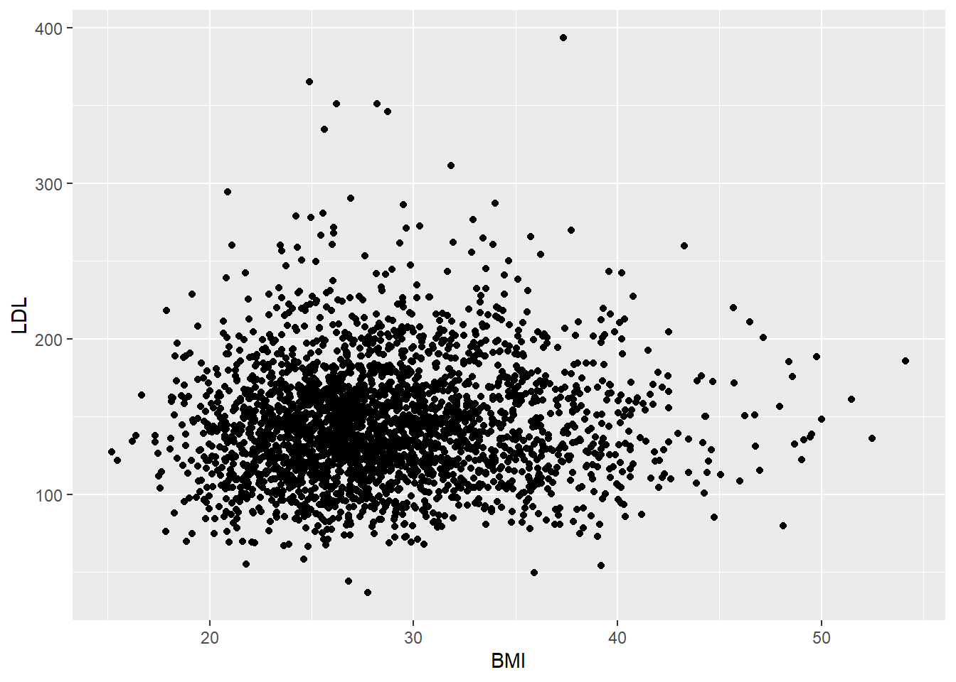
6.5 Case QQ
6.5.1 Numeric Summaries
The two most popular numeric summaries between two quantitative variables are
- correlation
- slope from a simple linear regression
We will only look at the correlation. Linear regression will be covered in Chapter 11.
We can obtain either Pearson’s correlation or Spearman’s rank correlation by using the cor function. To handle missing values, set the use option in cor to one of “complete.obs” or “pairwise.complete.obs”. Complete.obs uses data only from rows that are fully observed (none of the variables are missing for that observation) while pairwise.complete.obs only checks that both of the variables currently being studied are observed.
[1] 0.06066435[1] 0.06582967
6.6 Exercises
For these exercises, we will use the bike lanes dataset (source), Bike_Lanes.csv. You can download this dataset from the course webpage.
- How many bike lanes are currently in Baltimore? You can assume that each observation/row is a different bike lane.
- How many (a) feet and (b) miles of total bike lanes are currently in Baltimore? (The
lengthvariable provides the length in feet.) - How many types (
type) bike lanes are there? Which type (a) occurs the most and (b) has the longest average bike lane length? - How many different projects (
project) do the bike lanes fall into? Whichprojectcategory has the longest average bike lane length? - What was the average bike lane length per year that they were installed? (Be sure to first set
dateInstalledtoNAif it is equal to zero.) - Numerically and (b) graphically describe the distribution of bike lane lengths (
length).
- Numerically and (b) graphically describe the distribution of bike lane lengths (
- Describe the distribution of bike lane lengths numerically and graphically after stratifying them by (a) type and then by (b) number of lanes (
numLanes).