Chapter 16 Solutions to Exercises
16.1 RStudio
- Go through and change the colors in
paletteto something other than what they originally were. See http://www.stat.columbia.edu/~tzheng/files/Rcolor.pdf for a large list of colors. - Change the days you are keeping to show
"Sunday"instead of"Saturday". - Change the word
geom_line()togeom_point().
# keep only some days
avg = avg %>%
  filter(day %in% c("Monday", "Tuesday", "Friday", "Sunday")) #change Saturday to Sunday
filter: removed 1,237 rows (43%), 1,647 rows remaining# Modify these colors to something else
palette = c(
banner = "red",
green = "yellow",
orange = "darkblue",
purple = "brown")
ggplot(aes(x = date, y = number, colour = line), data= avg) +
geom_point() + #change this to geom_point()
facet_wrap( ~day) +
scale_colour_manual(values = palette)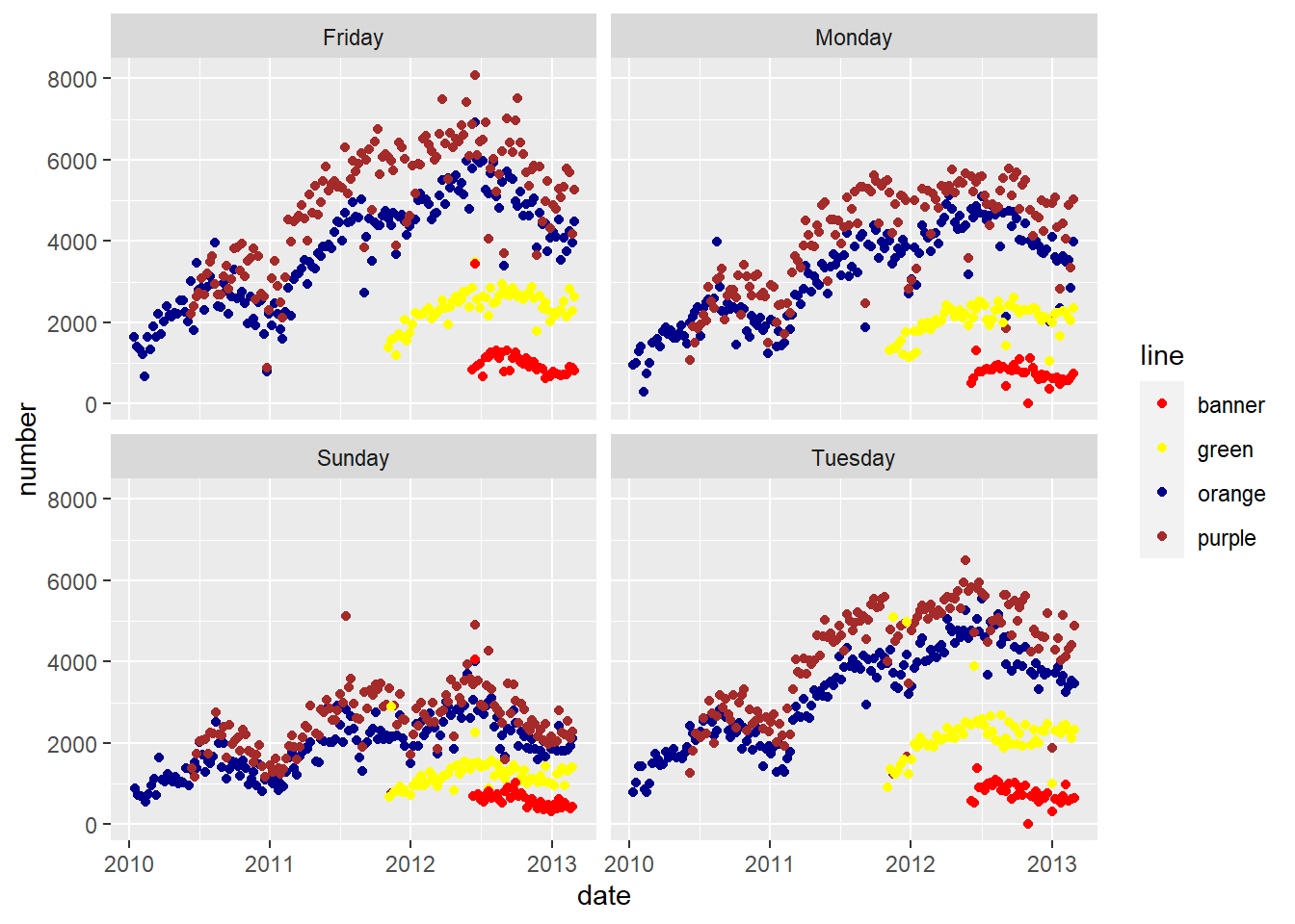
16.2 Basic R
- create a new variable called
my.numthat contains 6 numbers
- multiply
my.numby 4
[1] 20 16 28 32 48 56- create a second variable called
my.charthat contains 5 character strings
- combine the two variables
my.numandmy.charinto a variable calledboth
- what is the length of
both?
[1] 11- what class is
both?
[1] "character"- divide
bothby 3, what happens?
Error in both/3: non-numeric argument to binary operator- create a vector with elements 1 2 3 4 5 6 and call it
x
- create another vector with elements 10 20 30 40 50 and call it
y
- what happens if you try to add
xandytogether? why?
[1] 11 22 33 44 55 16Since y is shorter than x, it “recycles” the first element if y to make it long enough to match the length of x. This is can be a useful trick, but you must be careful when using R’s recycling.
11. append the value 60 onto the vector y (hint: you can use the c() function)
- add
xandytogether
[1] 11 22 33 44 55 66- multiply
xandytogether. pay attention to how R performs operations on vectors of the same length.
[1] 10 40 90 160 250 360Note that R does vector operations componentwise.
16.3 Data IO
- Read in the Youth Tobacco study, Youth_Tobacco_Survey_YTS_Data.csv and name it
youth.
Rows: 9794 Columns: 31
── Column specification ──────────────────────────────────────────────
Delimiter: ","
chr (24): LocationAbbr, LocationDesc, TopicType, TopicDesc, MeasureDesc, Dat...
dbl  (7): YEAR, Data_Value, Data_Value_Std_Err, Low_Confidence_Limit, High_C...

ℹ Use `spec()` to retrieve the full column specification for this data.
ℹ Specify the column types or set `show_col_types = FALSE` to quiet this message.- Install and invoke the
readxlpackage. RStudio > Tools > Install Packages. Type readxl into the Package search and click install. Load the installed library withlibrary(readxl).
- Download an Excel version of the Monuments dataset, Monuments.xlsx, from CANVAS. Use the
read_excel()function in thereadxlpackage to read in the dataset and call the outputmon.
- Write out the
monR object as a CSV file usingreadr::write_csvand call the file “monuments.csv”.
- Write out the
monR object as an RDS file usingreadr::write_rdsand call it “monuments.rds”.
16.4 Subsetting Data
- Check to see if you have the
mtcarsdataset by entering the commandmtcars.
                   mpg cyl disp  hp drat    wt  qsec vs am gear carb
Mazda RX4         21.0   6  160 110 3.90 2.620 16.46  0  1    4    4
Mazda RX4 Wag     21.0   6  160 110 3.90 2.875 17.02  0  1    4    4
Datsun 710        22.8   4  108  93 3.85 2.320 18.61  1  1    4    1
Hornet 4 Drive    21.4   6  258 110 3.08 3.215 19.44  1  0    3    1
Hornet Sportabout 18.7   8  360 175 3.15 3.440 17.02  0  0    3    2
Valiant 18.1 6 225 105 2.76 3.460 20.22 1 0 3 1- What class is
mtcars?
[1] "data.frame"- How many observations (rows) and variables (columns) are in the
mtcarsdataset?
[1] 32 11[1] 32[1] 11Rows: 32
Columns: 11
$ mpg <dbl> 21.0, 21.0, 22.8, 21.4, 18.7, 18.1, 14.3, 24.4, 22.8, 19.2, 17.8,…
$ cyl <dbl> 6, 6, 4, 6, 8, 6, 8, 4, 4, 6, 6, 8, 8, 8, 8, 8, 8, 4, 4, 4, 4, 8,…
$ disp <dbl> 160.0, 160.0, 108.0, 258.0, 360.0, 225.0, 360.0, 146.7, 140.8, 16…
$ hp <dbl> 110, 110, 93, 110, 175, 105, 245, 62, 95, 123, 123, 180, 180, 180…
$ drat <dbl> 3.90, 3.90, 3.85, 3.08, 3.15, 2.76, 3.21, 3.69, 3.92, 3.92, 3.92,…
$ wt <dbl> 2.620, 2.875, 2.320, 3.215, 3.440, 3.460, 3.570, 3.190, 3.150, 3.…
$ qsec <dbl> 16.46, 17.02, 18.61, 19.44, 17.02, 20.22, 15.84, 20.00, 22.90, 18…
$ vs <dbl> 0, 0, 1, 1, 0, 1, 0, 1, 1, 1, 1, 0, 0, 0, 0, 0, 0, 1, 1, 1, 1, 0,…
$ am <dbl> 1, 1, 1, 0, 0, 0, 0, 0, 0, 0, 0, 0, 0, 0, 0, 0, 0, 1, 1, 1, 0, 0,…
$ gear <dbl> 4, 4, 4, 3, 3, 3, 3, 4, 4, 4, 4, 3, 3, 3, 3, 3, 3, 4, 4, 4, 3, 3,…
$ carb <dbl> 4, 4, 1, 1, 2, 1, 4, 2, 2, 4, 4, 3, 3, 3, 4, 4, 4, 1, 2, 1, 1, 2,…- Copy
mtcarsinto an object called cars and renamempgin cars toMPG. Userename().
# A tibble: 6 × 11
    MPG   cyl  disp    hp  drat    wt  qsec    vs    am  gear  carb
  <dbl> <dbl> <dbl> <dbl> <dbl> <dbl> <dbl> <dbl> <dbl> <dbl> <dbl>
1  21       6   160   110  3.9   2.62  16.5     0     1     4     4
2  21       6   160   110  3.9   2.88  17.0     0     1     4     4
3  22.8     4   108    93  3.85  2.32  18.6     1     1     4     1
4  21.4     6   258   110  3.08  3.22  19.4     1     0     3     1
5  18.7     8   360   175  3.15  3.44  17.0     0     0     3     2
6 18.1 6 225 105 2.76 3.46 20.2 1 0 3 1- Convert the column names of
carsto all upper case. Userename_all, and thetouppercommand (orcolnames).
rename_all: renamed 10 variables (CYL, DISP, HP, DRAT, WT, …)# A tibble: 6 × 11
MPG CYL DISP HP DRAT WT QSEC VS AM GEAR CARB
<dbl> <dbl> <dbl> <dbl> <dbl> <dbl> <dbl> <dbl> <dbl> <dbl> <dbl>
1 21 6 160 110 3.9 2.62 16.5 0 1 4 4
2 21 6 160 110 3.9 2.88 17.0 0 1 4 4
3 22.8 4 108 93 3.85 2.32 18.6 1 1 4 1
4 21.4 6 258 110 3.08 3.22 19.4 1 0 3 1
5 18.7 8 360 175 3.15 3.44 17.0 0 0 3 2
6 18.1 6 225 105 2.76 3.46 20.2 1 0 3 1# Method 2
cars = as_tibble(mtcars)
cn = colnames(cars) # extract column names
cn = toupper(cn) # make them uppercase
colnames(cars) = cn # reassign
head(cars)# A tibble: 6 × 11
MPG CYL DISP HP DRAT WT QSEC VS AM GEAR CARB
<dbl> <dbl> <dbl> <dbl> <dbl> <dbl> <dbl> <dbl> <dbl> <dbl> <dbl>
1 21 6 160 110 3.9 2.62 16.5 0 1 4 4
2 21 6 160 110 3.9 2.88 17.0 0 1 4 4
3 22.8 4 108 93 3.85 2.32 18.6 1 1 4 1
4 21.4 6 258 110 3.08 3.22 19.4 1 0 3 1
5 18.7 8 360 175 3.15 3.44 17.0 0 0 3 2
6 18.1 6 225 105 2.76 3.46 20.2 1 0 3 1- Convert the rownames of
carsto a column calledcarusingrownames_to_column. Subset the columns fromcarsthat end in"p"and call it pvars usingends_with().
                car  mpg cyl disp  hp drat    wt  qsec vs am gear carb
1         Mazda RX4 21.0   6  160 110 3.90 2.620 16.46  0  1    4    4
2     Mazda RX4 Wag 21.0   6  160 110 3.90 2.875 17.02  0  1    4    4
3        Datsun 710 22.8   4  108  93 3.85 2.320 18.61  1  1    4    1
4    Hornet 4 Drive 21.4   6  258 110 3.08 3.215 19.44  1  0    3    1
5 Hornet Sportabout 18.7   8  360 175 3.15 3.440 17.02  0  0    3    2
6 Valiant 18.1 6 225 105 2.76 3.460 20.22 1 0 3 1 car disp hp
1 Mazda RX4 160 110
2 Mazda RX4 Wag 160 110
3 Datsun 710 108 93
4 Hornet 4 Drive 258 110
5 Hornet Sportabout 360 175
6 Valiant 225 105- Create a subset
carsthat only contains the columns:wt,qsec, andhpand assign this object tocarsSub. What are the dimensions ofcarsSub? (Useselect()anddim().)
[1] 32 4- Convert the column names of
carsSubto all upper case. Userename_all(), andtoupper()(orcolnames()).
rename_all: renamed 4 variables (CAR, WT, QSEC, HP)- Subset the rows of
carsthat get more than 20 miles per gallon (mpg) of fuel efficiency. How many are there? (Usefilter().)
filter: removed 18 rows (56%), 14 rows remaining[1] 14 12[1] 14Rows: 14
Columns: 12
$ car <chr> "Mazda RX4", "Mazda RX4 Wag", "Datsun 710", "Hornet 4 Drive", "Me…
$ mpg <dbl> 21.0, 21.0, 22.8, 21.4, 24.4, 22.8, 32.4, 30.4, 33.9, 21.5, 27.3,…
$ cyl <dbl> 6, 6, 4, 6, 4, 4, 4, 4, 4, 4, 4, 4, 4, 4
$ disp <dbl> 160.0, 160.0, 108.0, 258.0, 146.7, 140.8, 78.7, 75.7, 71.1, 120.1…
$ hp <dbl> 110, 110, 93, 110, 62, 95, 66, 52, 65, 97, 66, 91, 113, 109
$ drat <dbl> 3.90, 3.90, 3.85, 3.08, 3.69, 3.92, 4.08, 4.93, 4.22, 3.70, 4.08,…
$ wt <dbl> 2.620, 2.875, 2.320, 3.215, 3.190, 3.150, 2.200, 1.615, 1.835, 2.…
$ qsec <dbl> 16.46, 17.02, 18.61, 19.44, 20.00, 22.90, 19.47, 18.52, 19.90, 20…
$ vs <dbl> 0, 0, 1, 1, 1, 1, 1, 1, 1, 1, 1, 0, 1, 1
$ am <dbl> 1, 1, 1, 0, 0, 0, 1, 1, 1, 0, 1, 1, 1, 1
$ gear <dbl> 4, 4, 4, 3, 4, 4, 4, 4, 4, 3, 4, 5, 5, 4
$ carb <dbl> 4, 4, 1, 1, 2, 2, 1, 2, 1, 1, 1, 2, 2, 2There are 14 cars. There are now nrow(cars_mpg) cars.
filter: removed 18 rows (56%), 14 rows remaining[1] 14filter: removed 18 rows (56%), 14 rows remaining[1] 14- Subset the rows that get less than 16 miles per gallon (
mpg) of fuel efficiency and have more than 100 horsepower (hp). How many are there? (Usefilter().)
filter: removed 22 rows (69%), 10 rows remaining car mpg cyl disp hp drat wt qsec vs am gear carb
1 Duster 360 14.3 8 360.0 245 3.21 3.570 15.84 0 0 3 4
2 Merc 450SLC 15.2 8 275.8 180 3.07 3.780 18.00 0 0 3 3
3 Cadillac Fleetwood 10.4 8 472.0 205 2.93 5.250 17.98 0 0 3 4
4 Lincoln Continental 10.4 8 460.0 215 3.00 5.424 17.82 0 0 3 4
5 Chrysler Imperial 14.7 8 440.0 230 3.23 5.345 17.42 0 0 3 4
6 Dodge Challenger 15.5 8 318.0 150 2.76 3.520 16.87 0 0 3 2
7 AMC Javelin 15.2 8 304.0 150 3.15 3.435 17.30 0 0 3 2
8 Camaro Z28 13.3 8 350.0 245 3.73 3.840 15.41 0 0 3 4
9 Ford Pantera L 15.8 8 351.0 264 4.22 3.170 14.50 0 1 5 4
10 Maserati Bora 15.0 8 301.0 335 3.54 3.570 14.60 0 1 5 8filter: removed 22 rows (69%), 10 rows remaining[1] 10filter: removed 22 rows (69%), 10 rows remaining[1] 10filter: removed 22 rows (69%), 10 rows remaining[1] 10- Create a subset of the
carsdata that only contains the columns:wt,qsec, andhpfor cars with 8 cylinders (cyl) and reassign this object tocarsSub. What are the dimensions of this dataset?
filter: removed 18 rows (56%), 14 rows remaining[1] 14 4filter: removed 18 rows (56%), 14 rows remaining[1] 14 4- Re-order the rows of
carsSubby weight (wt) in increasing order. (Usearrange().)
- Create a new variable in
carsSubcalledwt2, which is equal towt^2, usingmutate()and piping%>%.
      wt  qsec  hp                 car      wt2
1  3.170 14.50 264      Ford Pantera L 10.04890
2  3.435 17.30 150         AMC Javelin 11.79922
3  3.440 17.02 175   Hornet Sportabout 11.83360
4  3.520 16.87 150    Dodge Challenger 12.39040
5  3.570 15.84 245          Duster 360 12.74490
6  3.570 14.60 335       Maserati Bora 12.74490
7  3.730 17.60 180          Merc 450SL 13.91290
8  3.780 18.00 180         Merc 450SLC 14.28840
9  3.840 15.41 245          Camaro Z28 14.74560
10 3.845 17.05 175    Pontiac Firebird 14.78403
11 4.070 17.40 180          Merc 450SE 16.56490
12 5.250 17.98 205  Cadillac Fleetwood 27.56250
13 5.345 17.42 230   Chrysler Imperial 28.56902
14 5.424 17.82 215 Lincoln Continental 29.41978
16.5 Data Summarization
- How many bike lanes are currently in Baltimore? You can assume that each observation/row is a different bike lane.
[1] 1631[1] 1631 9[1] 1631- How many (a) feet and (b) miles of total bike lanes are currently in Baltimore? (The
lengthvariable provides the length in feet.)
[1] 439447.6[1] 83.22871[1] 83.22871- How many types (
type) bike lanes are there? Which type (a) occurs the most and (b) has the longest average bike lane length?
 BIKE BOULEVARD       BIKE LANE      CONTRAFLOW SHARED BUS BIKE         SHARROW
             49             621              13              39             589
       SIDEPATH    SIGNED ROUTE            <NA>
7 304 9 [1] "BIKE BOULEVARD" "SIDEPATH" "SIGNED ROUTE" "BIKE LANE"
[5] "SHARROW" NA "CONTRAFLOW" "SHARED BUS BIKE"[1] 7[1] 8[1] FALSE FALSE FALSE FALSE FALSE TRUE FALSE FALSEcount: now 8 rows and 2 columns, ungrouped# (b)
bike %>%
group_by(type) %>%
summarise(number_of_rows = n(),
mean = mean(length)) %>%
arrange(desc(mean))summarise: now 8 rows and 3 columns, ungrouped# A tibble: 8 × 3
type number_of_rows mean
<chr> <int> <dbl>
1 SIDEPATH 7 666.
2 BIKE LANE 621 300.
3 SHARED BUS BIKE 39 277.
4 SIGNED ROUTE 304 264.
5 <NA> 9 260.
6 SHARROW 589 244.
7 BIKE BOULEVARD 49 197.
8 CONTRAFLOW 13 136.- How many different projects (
project) do the bike lanes fall into? Whichprojectcategory has the longest average bike lane length?
[1] 13# Several different solutions for finding the longest average bike lane length for a project
bike %>%
group_by(project) %>%
summarise(n = n(),
mean = mean(length)) %>%
arrange(desc(mean)) summarise: now 13 rows and 3 columns, ungrouped# A tibble: 13 × 3
project n mean
<chr> <int> <dbl>
1 MAINTENANCE 4 1942.
2 ENGINEERING CONSTRUCTION 12 512.
3 TRAFFIC 51 420.
4 COLLEGETOWN 339 321.
5 PARK HEIGHTS BIKE NETWORK 172 283.
6 CHARM CITY CIRCULATOR 39 277.
7 TRAFFIC CALMING 79 269.
8 OPERATION ORANGE CONE 458 250.
9 <NA> 74 214.
10 COLLEGETOWN NETWORK 13 214.
11 SOUTHEAST BIKE NETWORK 323 211.
12 PLANNING TRAFFIC 18 209.
13 GUILFORD AVE BIKE BLVD 49 197.bike %>%
group_by(project, type) %>%
summarise(n = n(),
mean = mean(length)) %>%
arrange(desc(mean)) %>%
ungroup() %>%
slice(1) %>%
magrittr::extract("project")summarise: now 32 rows and 4 columns, one group variable remaining (project)ungroup: no grouping variablesslice: removed 31 rows (97%), one row remaining# A tibble: 1 × 1
project
<chr>
1 MAINTENANCEsummarize: now 32 rows and 4 columns, one group variable remaining (project)# A tibble: 32 × 4
# Groups: project [13]
project type n mean
<chr> <chr> <int> <dbl>
1 MAINTENANCE BIKE LANE 4 1942.
2 TRAFFIC SIDEPATH 1 1848.
3 ENGINEERING CONSTRUCTION BIKE LANE 8 537.
4 <NA> SIDEPATH 2 512.
5 ENGINEERING CONSTRUCTION SIDEPATH 3 481.
6 ENGINEERING CONSTRUCTION SHARROW 1 403.
7 PARK HEIGHTS BIKE NETWORK SIGNED ROUTE 27 398.
8 TRAFFIC BIKE LANE 50 391.
9 PLANNING TRAFFIC BIKE LANE 6 363.
10 <NA> BIKE LANE 12 357.
# ℹ 22 more rowsavg = bike %>%
group_by(type) %>%
summarize(mn = mean(length, na.rm = TRUE)) %>%
filter(mn == max(mn))summarize: now 8 rows and 2 columns, ungroupedfilter: removed 7 rows (88%), one row remaining- What was the average bike lane length per year that they were installed? (Be sure to first set
dateInstalledtoNAif it is equal to zero.)
# Several example of changing 0's to NA for dateInstalled
bike = bike %>% mutate(
  dateInstalled = ifelse(
    dateInstalled == 0,
    NA,
    dateInstalled)
)
mean(bike$length[ !is.na(bike$dateInstalled)]) # overall average bike lane length
[1] 273.9943b2 = bike %>%
mutate(dateInstalled = ifelse(dateInstalled == "0", NA,
dateInstalled))
b2 = bike %>%
mutate(dateInstalled = if_else(dateInstalled == "0",
NA_real_,
dateInstalled))
bike$dateInstalled[bike$dateInstalled == "0"] = NA
# Mean bike lane length by year. Note that bike lane length of 0 is also NA
bike %>%
mutate(length = ifelse(length == 0, NA, length)) %>%
group_by(dateInstalled) %>%
summarise(n = n(),
mean_of_the_bike = mean(length, na.rm = TRUE),
n_missing = sum(is.na(length)))summarise: now 9 rows and 4 columns, ungrouped# A tibble: 9 × 4
dateInstalled n mean_of_the_bike n_missing
<dbl> <int> <dbl> <int>
1 2006 2 1469. 0
2 2007 368 310. 0
3 2008 206 249. 0
4 2009 86 407. 0
5 2010 625 246. 0
6 2011 101 233. 0
7 2012 107 271. 0
8 2013 10 290. 0
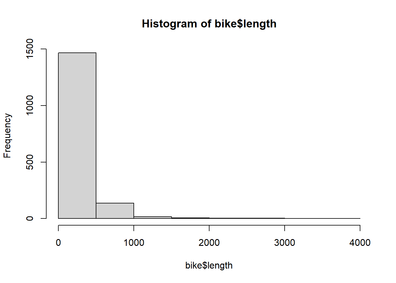
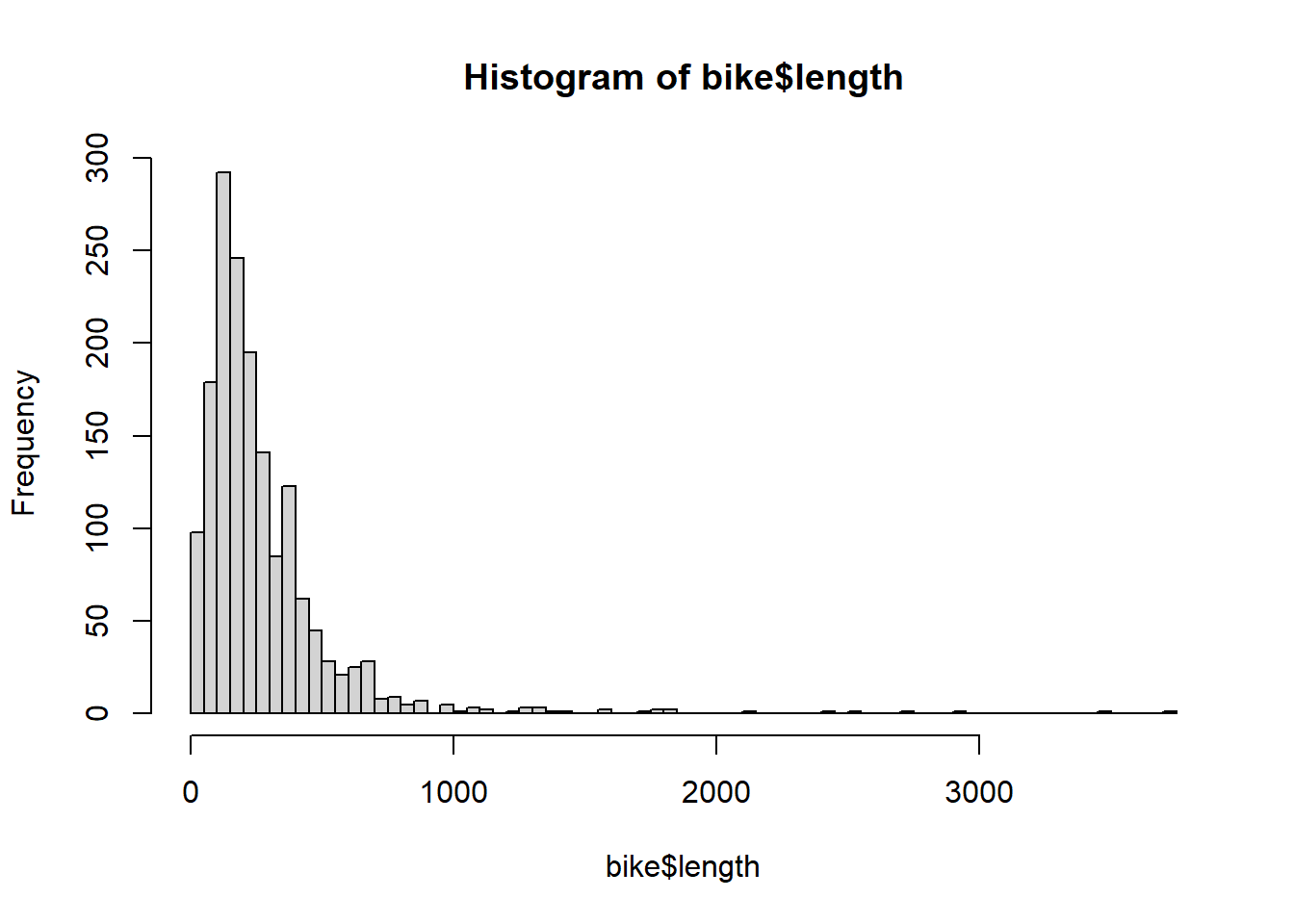
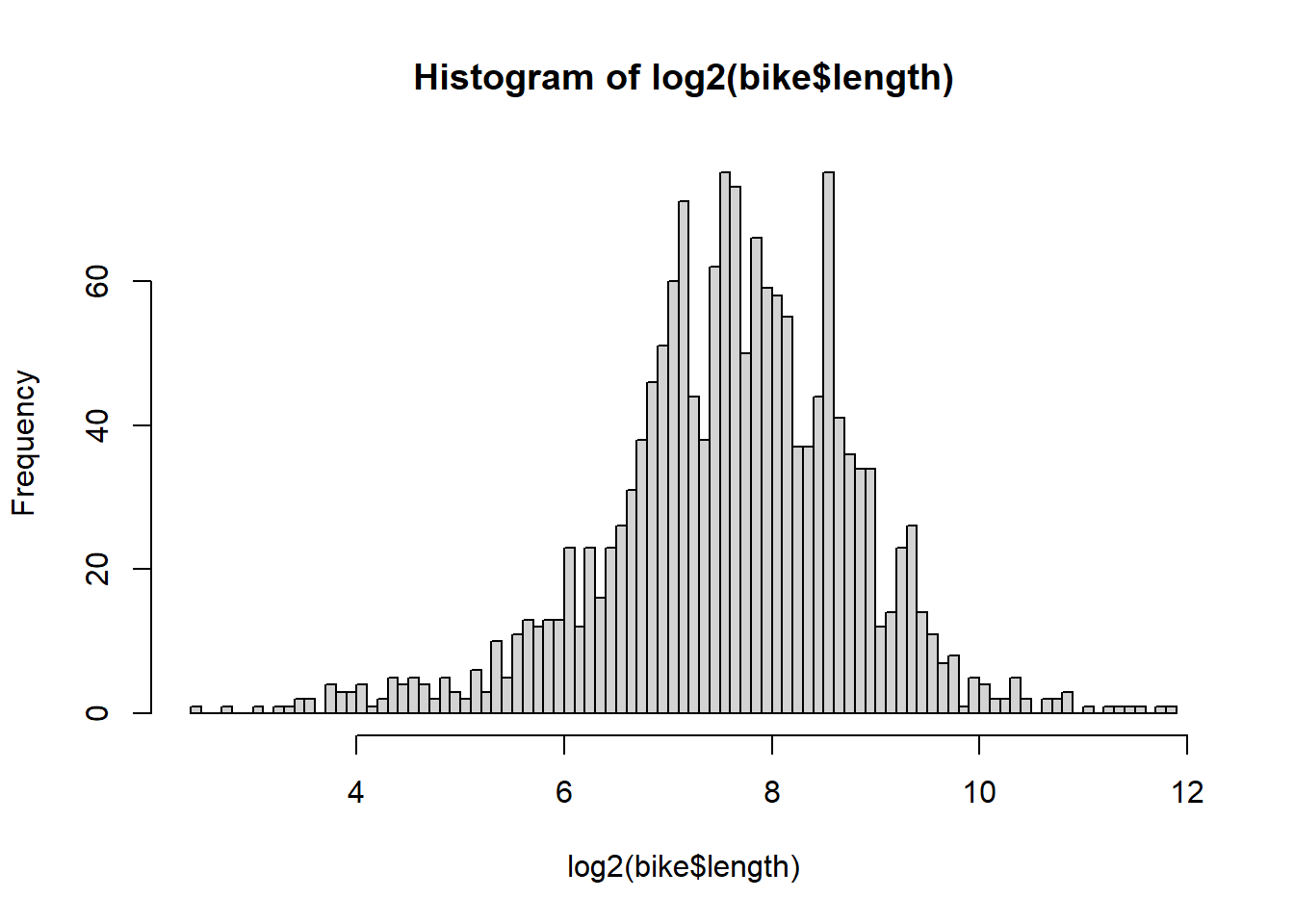
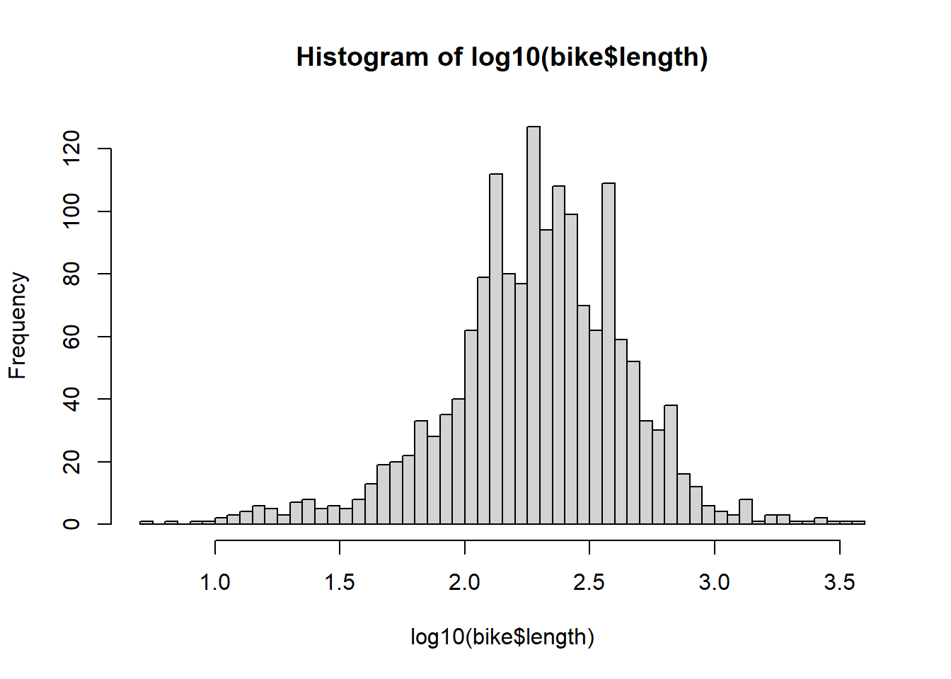
9 NA 126 217. 1- Numerically and (b) graphically describe the distribution of bike lane lengths (
length).
- Numerically and (b) graphically describe the distribution of bike lane lengths (
       0%       25%       50%       75%      100%
0.0000 124.0407 200.3027 341.0224 3749.3226 `stat_bin()` using `bins = 30`. Pick better value with `binwidth`.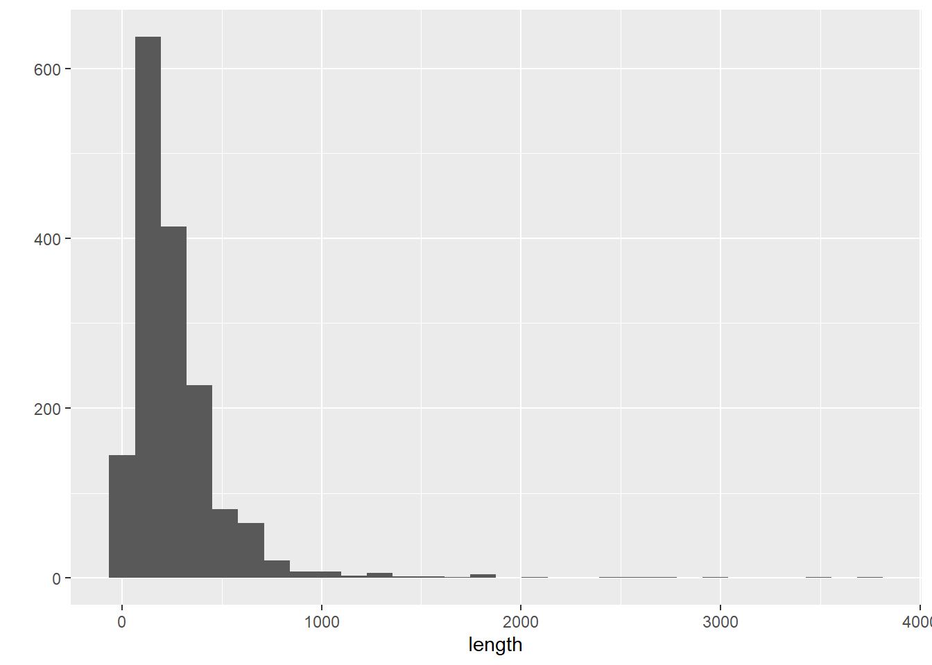
`stat_bin()` using `bins = 30`. Pick better value with `binwidth`.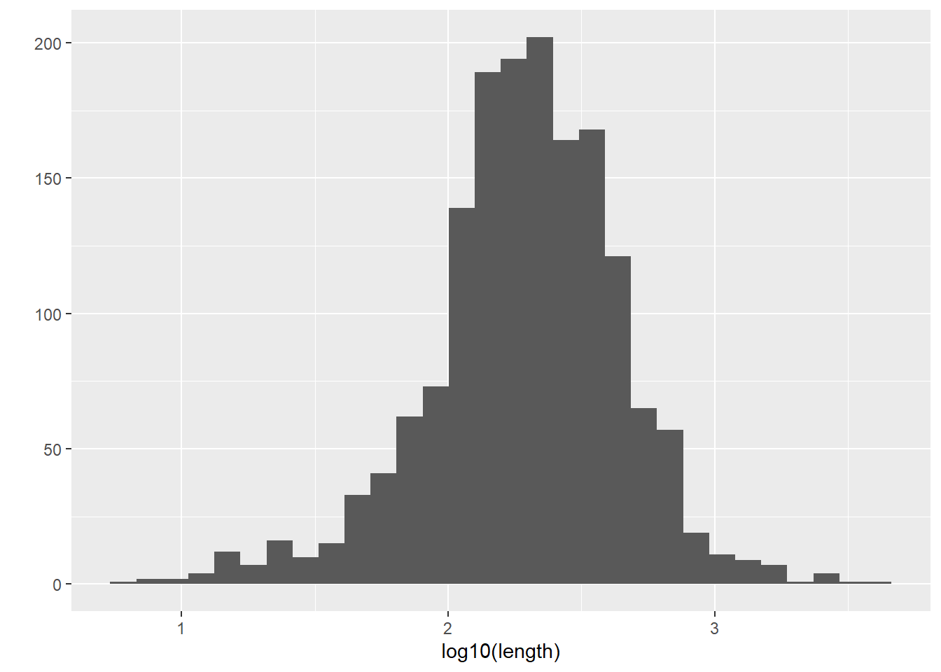
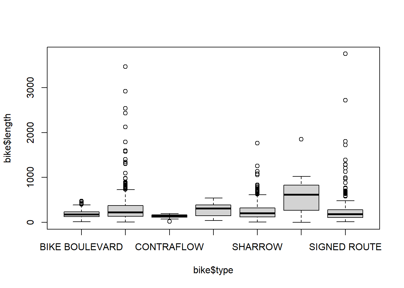
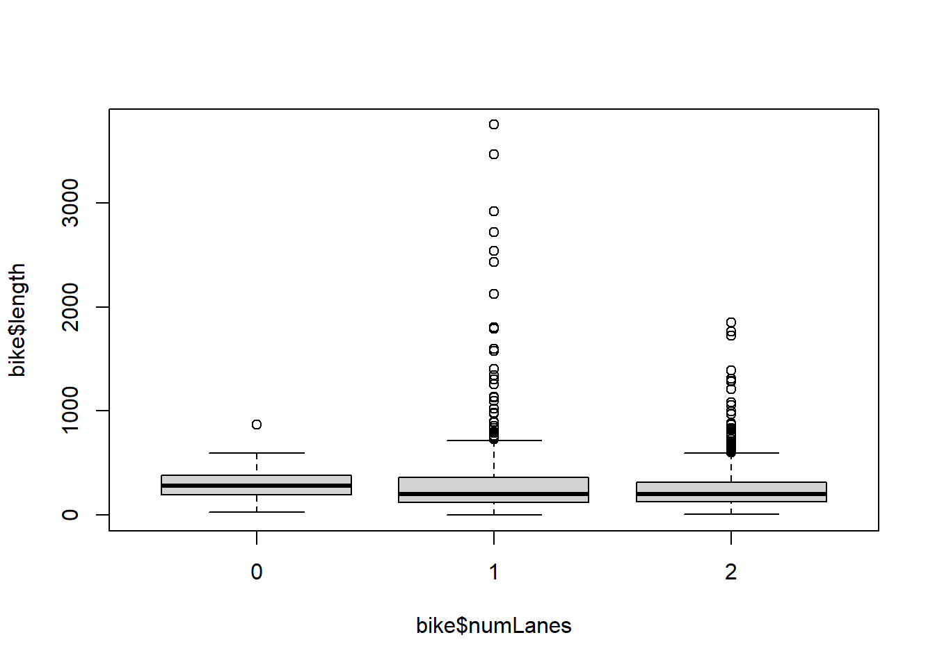
 7. Describe the distribution of bike lane lengths numerically and graphically after stratifying them by (a) type and then by (b) number of lanes (
numLanes).
# (a)
bike %>%
  group_by(type) %>%
  summarise(mean_length = mean(length, rm.na = TRUE),
            sd_length = sd(length, na.rm = TRUE))
summarise: now 8 rows and 3 columns, ungrouped# A tibble: 8 × 3
type mean_length sd_length
<chr> <dbl> <dbl>
1 BIKE BOULEVARD 197. 113.
2 BIKE LANE 300. 315.
3 CONTRAFLOW 136. 48.5
4 SHARED BUS BIKE 277. 140.
5 SHARROW 244. 188.
6 SIDEPATH 666. 619.
7 SIGNED ROUTE 264. 348.
8 <NA> 260. 254. 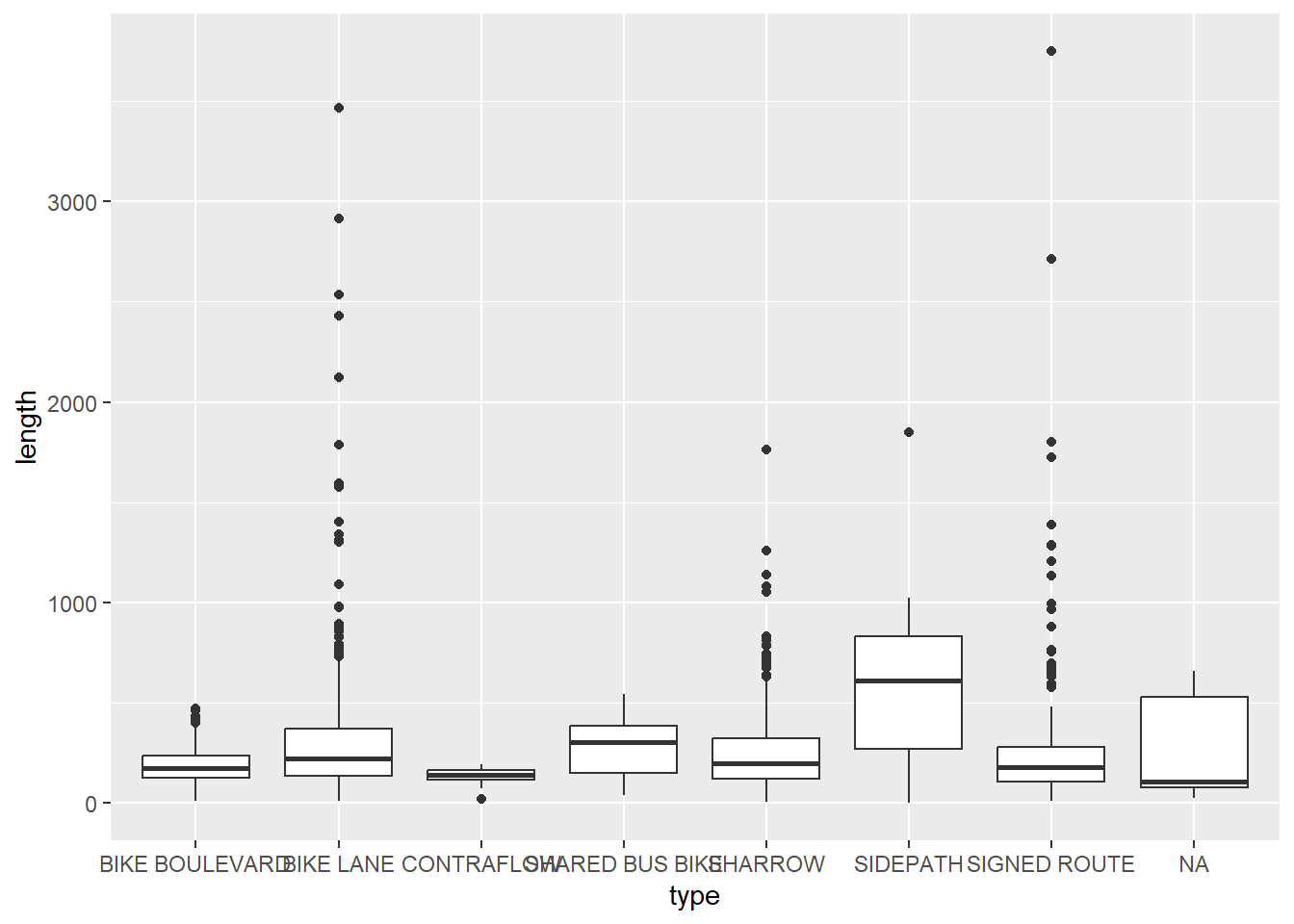
# (b)
bike %>%
  group_by(numLanes) %>%
  summarise(mean_length = mean(length, rm.na = TRUE),
            sd_length = sd(length, na.rm = TRUE))
summarise: now 3 rows and 3 columns, ungrouped# A tibble: 3 × 3
numLanes mean_length sd_length
<dbl> <dbl> <dbl>
1 0 308. 202.
2 1 278. 318.
3 2 258. 219.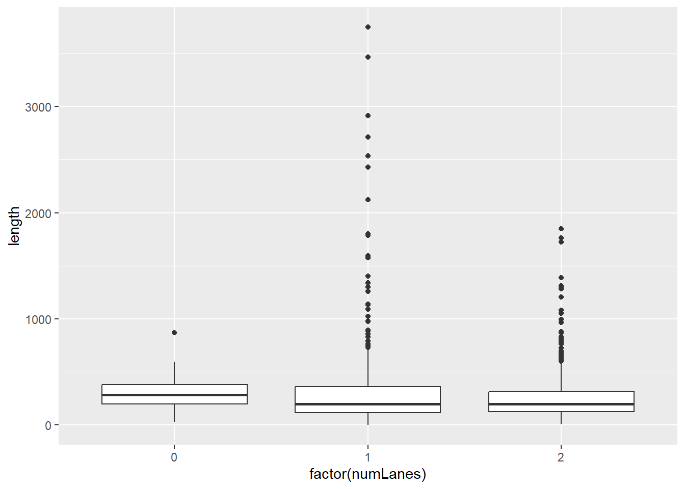
16.6 Data Classes
library(readr)
library(tidyverse)
library(dplyr)
library(lubridate)

bike = read_csv("./data/Bike_Lanes.csv")- Get all the different types of bike lanes from the
typecolumn. Usesort(unique()). Assign this to an objectbtypes. Typedput(btypes).
[1] BIKE BOULEVARD SIDEPATH       SIGNED ROUTE   SIDEPATH       BIKE LANE
[6] SIGNED ROUTE
7 Levels: BIKE BOULEVARD BIKE LANE CONTRAFLOW SHARED BUS BIKE ... SIGNED ROUTE
btypes = sort(unique(bike$type)) # get the unique categories in type. easier than typing them out as shown below in x
x = c("SIDEPATH","BIKE BOULEVARD", "BIKE LANE", "CONTRAFLOW",
"SHARED BUS BIKE", "SHARROW", "SIGNED ROUTE") #same vector as btypes
dput(btypes) #outputs the c() vector. can be used for assignc("BIKE BOULEVARD", "BIKE LANE", "CONTRAFLOW", "SHARED BUS BIKE",
"SHARROW", "SIDEPATH", "SIGNED ROUTE")- By rearranging vector
btypesand usingdput, recodetypeas a factor that hasSIDEPATHas the first level. Printhead(bike$type). Note what you see. Runtable(bike$type)afterwards and note the order.
c("BIKE BOULEVARD", "BIKE LANE", "CONTRAFLOW", "SHARED BUS BIKE",
"SHARROW", "SIDEPATH", "SIGNED ROUTE")[1] "SIDEPATH" "BIKE BOULEVARD" "BIKE LANE" "CONTRAFLOW"
[5] "SHARED BUS BIKE" "SHARROW" "SIGNED ROUTE" c("SIDEPATH", "BIKE BOULEVARD", "BIKE LANE", "CONTRAFLOW", "SHARED BUS BIKE",
"SHARROW", "SIGNED ROUTE")
 BIKE BOULEVARD       BIKE LANE      CONTRAFLOW SHARED BUS BIKE         SHARROW
             49             621              13              39             589
       SIDEPATH    SIGNED ROUTE
7 304 bike$type = relevel(bike$type, "SIDEPATH")
bike$type = factor(bike$type,
levels = dput(btypes[c(6,1:5,7)]))c("SIDEPATH", "BIKE BOULEVARD", "BIKE LANE", "CONTRAFLOW", "SHARED BUS BIKE",
"SHARROW", "SIGNED ROUTE")c("SIDEPATH", "BIKE BOULEVARD", "BIKE LANE", "CONTRAFLOW", "SHARED BUS BIKE",
"SHARROW", "SIGNED ROUTE")
       SIDEPATH  BIKE BOULEVARD       BIKE LANE      CONTRAFLOW SHARED BUS BIKE
              7              49             621              13              39
        SHARROW    SIGNED ROUTE
589 304 - Make a column called
type2, which is a factor of thetypecolumn, with the levels:c("SIDEPATH", "BIKE BOULEVARD", "BIKE LANE"). Runtable(bike$type2), with the optionsuseNA = "always". Note, we do not have to make type a character again before doing this.
bike = bike %>%
  mutate(type2 = factor(type,
             levels = c( "SIDEPATH", "BIKE BOULEVARD",
                         "BIKE LANE") ) )
table(bike$type)
       SIDEPATH  BIKE BOULEVARD       BIKE LANE      CONTRAFLOW SHARED BUS BIKE
              7              49             621              13              39
        SHARROW    SIGNED ROUTE
            589             304
      SIDEPATH BIKE BOULEVARD      BIKE LANE
7 49 621 table(bike$type2, useNA = "always") #The other levels are now counted as NA since they are not included in the levels
      SIDEPATH BIKE BOULEVARD      BIKE LANE           <NA>
7 49 621 954 - Reassign
dateInstalledinto a character usingas.character. Runhead(bike$dateInstalled).
- Reassign
[1] "0" "2010" "2010" "0" "2011" "2007"b. Reassign `dateInstalled` as a factor, using the default levels. Run `head(bike$dateInstalled)`. [1] 0 2010 2010 0 2011 2007
Levels: 0 2006 2007 2008 2009 2010 2011 2012 2013
2005 2006 2007 2008 2009 2010 2011 2012 2013 2014 2015 2016 2017
   0    2  368  206   86  625  101  107   10    0    0    0    0
2005 2006 2007 2008 2009 2010 2011 2012 2013 2014 2015 2016 2017 <NA>
   0    2  368  206   86  625  101  107   10    0    0    0    0  126
c. Do not reassign `dateInstalled`, but simply run `head(as.numeric(bike$dateInstalled))`. We are looking to see what happens when we try to go from factor to numeric. [1] 1 6 6 1 7 3d. Do not reassign `dateInstalled`, but simply run `head(as.numeric(as.character(bike$dateInstalled)))`. This is how you get a "numeric" value back if they were incorrectly converted to factors.[1] 0 2010 2010 0 2011 2007- Convert
typeback to a character vector. Make a columntype2(replacing the old one), where if the type is one of these categoriesc("CONTRAFLOW", "SHARED BUS BIKE", "SHARROW", "SIGNED ROUTE")call it"OTHER". Use%in%andifelse. Maketype2a factor with the levelsc("SIDEPATH", "BIKE BOULEVARD", "BIKE LANE", "OTHER").
# Note that this is done in a single mutate but the order matters
bike = bike %>% mutate(
    type = as.character(type),
    type2 = ifelse(type %in% c("CONTRAFLOW", "SHARED BUS BIKE",
                               "SHARROW", "SIGNED ROUTE"), "OTHER", type),
    type2 = factor(type2, levels = c( "SIDEPATH", "BIKE BOULEVARD",
                               "BIKE LANE", "OTHER") ))

table(bike$type2)
      SIDEPATH BIKE BOULEVARD      BIKE LANE          OTHER
             7             49            621            945
# An alternative way to recode type2
bike2 = bike %>%
mutate(
type = factor(type,
levels = c( "SIDEPATH", "BIKE BOULEVARD",
"BIKE LANE", "CONTRAFLOW",
"SHARED BUS BIKE",
"SHARROW", "SIGNED ROUTE")
),
type2 = recode_factor(type,
"CONTRAFLOW" = "OTHER",
"SHARED BUS BIKE" = "OTHER",
"SHARROW" = "OTHER",
"SIGNED ROUTE" = "OTHER")
)
table(bike2$type2)
         OTHER       SIDEPATH BIKE BOULEVARD      BIKE LANE
945 7 49 621 - Parse the following dates using the correct
lubridatefunctions:- “2014/02-14”
[1] "2014-02-14"b. "04/22/14 03:20" assume `mdy`[1] "2014-04-22 03:20:00 UTC"c. “4/5/2016 03:2:22” assume `mdy`[1] "2016-04-05 03:02:22 UTC"16.7 Data Cleaning
library(readr)
library(tidyverse)
library(dplyr)
library(lubridate)
library(tidyverse)
library(broom)

bike = read_csv("./data/Bike_Lanes.csv")- Count the number of rows of the bike data and count the number of complete cases of the bike data. Use
sumandcomplete.cases.
[1] 1631[1] 257- Create a data set called namat which is equal to
is.na(bike). What is the class ofnamat? RunrowSumsandcolSumsonnamat. These represent the number of missing values in the rows and columns of bike. Don’t printrowSums, but do a table of therowSums.
[1] "matrix" "array" subType name block type numLanes
4 12 215 9 0
project route length dateInstalled
74 1269 0 0
   0    1    2    3    4
257 1181 182 6 5 - Filter rows of bike that are NOT missing the
routevariable, assign this to the objecthave_route. Do a table of thesubTypevariable using table, including the missingsubTypes. Get the same frequency distribution usinggroup_by(subType)andtally()orcount().
filter: removed 1,269 rows (78%), 362 rows remaining[1] 362 9
STRALY STRPRD   <NA>
3 358 1 tally: now 3 rows and 2 columns, ungrouped# A tibble: 3 × 2
subType n
<chr> <int>
1 STRALY 3
2 STRPRD 358
3 <NA> 1count: now 3 rows and 2 columns, one group variable remaining (subType)# A tibble: 3 × 2
# Groups: subType [3]
subType n
<chr> <int>
1 STRALY 3
2 STRPRD 358
3 <NA> 1summarize: now 3 rows and 2 columns, ungrouped# A tibble: 3 × 2
subType n_obs
<chr> <int>
1 STRALY 3
2 STRPRD 358
3 <NA> 1tally: now 3 rows and 2 columns, ungrouped# A tibble: 3 × 2
subType n
<chr> <int>
1 STRALY 3
2 STRPRD 358
3 <NA> 1tally: now 3 rows and 2 columns, ungrouped# A tibble: 3 × 2
subType n
<chr> <int>
1 STRALY 3
2 STRPRD 358
3 <NA> 1- Filter rows of
bikethat have the typeSIDEPATHorBIKE LANEusing%in%. Call itside_bike. Confirm this gives you the same number of results using the|and==.
filter: removed 1,003 rows (61%), 628 rows remainingfilter: removed 1,003 rows (61%), 628 rows remaining[1] TRUE[1] 628[1] 628filter: removed 1,003 rows (61%), 628 rows remainingfilter: removed 1,003 rows (61%), 628 rows remaining[1] TRUE- Do a cross tabulation of the bike
typeand the number of lanes (numLanes). Call ittab. Do aprop.tableon the rows and columns margins. Tryas.data.frame(tab)orbroom::tidy(tab).
                 numLanes
type                       0          1          2
  BIKE BOULEVARD  0.00000000 0.02040816 0.97959184
  BIKE LANE       0.03220612 0.66183575 0.30595813
  CONTRAFLOW      0.00000000 0.53846154 0.46153846
  SHARED BUS BIKE 0.00000000 1.00000000 0.00000000
  SHARROW         0.00000000 0.36842105 0.63157895
  SIDEPATH        0.00000000 0.85714286 0.14285714
SIGNED ROUTE 0.00000000 0.69407895 0.30592105 numLanes
type 0 1 2
BIKE BOULEVARD 0.000000000 0.001121076 0.067605634
BIKE LANE 1.000000000 0.460762332 0.267605634
CONTRAFLOW 0.000000000 0.007847534 0.008450704
SHARED BUS BIKE 0.000000000 0.043721973 0.000000000
SHARROW 0.000000000 0.243273543 0.523943662
SIDEPATH 0.000000000 0.006726457 0.001408451
SIGNED ROUTE 0.000000000 0.236547085 0.130985915 type numLanes Freq
1 BIKE BOULEVARD 0 0
2 BIKE LANE 0 20
3 CONTRAFLOW 0 0
4 SHARED BUS BIKE 0 0
5 SHARROW 0 0
6 SIDEPATH 0 0
7 SIGNED ROUTE 0 0
8 BIKE BOULEVARD 1 1
9 BIKE LANE 1 411
10 CONTRAFLOW 1 7
11 SHARED BUS BIKE 1 39
12 SHARROW 1 217
13 SIDEPATH 1 6
14 SIGNED ROUTE 1 211
15 BIKE BOULEVARD 2 48
16 BIKE LANE 2 190
17 CONTRAFLOW 2 6
18 SHARED BUS BIKE 2 0
19 SHARROW 2 372
20 SIDEPATH 2 1
21 SIGNED ROUTE 2 93# A tibble: 21 × 3
type numLanes n
<chr> <chr> <int>
1 BIKE BOULEVARD 0 0
2 BIKE LANE 0 20
3 CONTRAFLOW 0 0
4 SHARED BUS BIKE 0 0
5 SHARROW 0 0
6 SIDEPATH 0 0
7 SIGNED ROUTE 0 0
8 BIKE BOULEVARD 1 1
9 BIKE LANE 1 411
10 CONTRAFLOW 1 7
# ℹ 11 more rows- Read the Property Tax data into R and call it the variable
tax.
- How many addresses pay property
taxes? (Assume each row is a different address.)
[1] 237963 16[1] 237963[1] 237963[1] 18696[1] 219267- What is the total (a) city (
CityTax) and (b) state (SateTax) tax paid? You need to remove the$from theCityTaxvariable, then you need to make it numeric. Trystr_replace, but remember$is “special” and you needfixed()around it.
[1] NA NA "$1463.45" "$2861.70" "$884.21" "$1011.60"tax = tax %>%
mutate(
CityTax = str_replace(CityTax,
fixed("$"), "") ,
CityTax = as.numeric(CityTax)
)
# no piping
tax$CityTax = str_replace(tax$CityTax, fixed("$"), "")
tax$CityTax = as.numeric(tax$CityTax)
sum(tax$CityTax) #there are NAs[1] NA[1] 831974818[1] 831.9748# (b)
options(digits=12) # so no rounding
tax = tax %>% mutate(StateTax = parse_number(StateTax))
sum(tax$StateTax, na.rm = TRUE) [1] 42085409.8[1] 42.0854098- Using
table()orgroup_byandsummarize(n())ortally().- How many observations/properties are in each ward (
Ward)?
- How many observations/properties are in each ward (
   01    02    03    04    05    06    07    08    09    10    11    12    13
 6613  3478  2490  1746   466  4360  4914 11445 11831  1704  3587  8874  9439
   14    15    16    17    18    19    20    21    22    23    24    25    26
 3131 18663 11285  1454  2314  3834 11927  3182  1720  2577  6113 14865 25510
   27    28    50
50215 10219 7 tally: now 29 rows and 2 columns, ungroupedsummarize: now 29 rows and 2 columns, ungroupedb. What is the mean state tax per ward? Use `group_by` and `summarize`.summarize: now 29 rows and 2 columns, ungrouped# A tibble: 29 × 2
Ward `mean(StateTax, na.rm = TRUE)`
<chr> <dbl>
1 01 291.
2 02 344.
3 03 726.
4 04 2327.
5 05 351.
6 06 178.
7 07 90.3
8 08 55.3
9 09 89.4
10 10 82.2
# ℹ 19 more rowsc. What is the maximum amount still due (`AmountDue`) in each ward? Use `group_by` and `summarize` with 'max`.tax = tax %>%
mutate(
AmountDue = str_replace(AmountDue,
fixed("$"), "") ,
AmountDue = as.numeric(AmountDue)
)
tax %>%
group_by(Ward) %>%
summarize(max_due = max(AmountDue, na.rm = TRUE))summarize: now 29 rows and 2 columns, ungrouped# A tibble: 29 × 2
Ward max_due
<chr> <dbl>
1 01 610032.
2 02 1459942.
3 03 1023666.
4 04 3746356.
5 05 948503.
6 06 407589.
7 07 1014574.
8 08 249133.
9 09 150837.
10 10 156216.
# ℹ 19 more rowsd. What is the 75th percentile of city and state tax paid by Ward? (`quantile`)summarize: now 29 rows and 2 columns, ungrouped# A tibble: 29 × 2
Ward Percentile
<chr> <dbl>
1 01 311.
2 02 321.
3 03 305.
4 04 569.
5 05 131.
6 06 195.
7 07 40.3
8 08 84.1
9 09 135.
10 10 101.
# ℹ 19 more rows# putting it all together
ward_table = tax %>%
group_by(Ward) %>%
summarize(
number_of_obs = n(),
mean_state_tax = mean(StateTax, na.rm = TRUE),
max_amount_due = max(AmountDue, na.rm = TRUE),
q75_city = quantile(CityTax, probs = 0.75, na.rm = TRUE),
q75_state = quantile(StateTax, probs = 0.75, na.rm = TRUE)
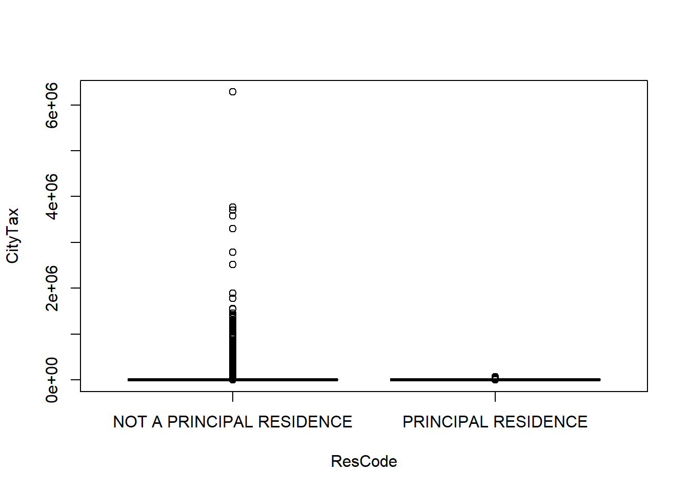
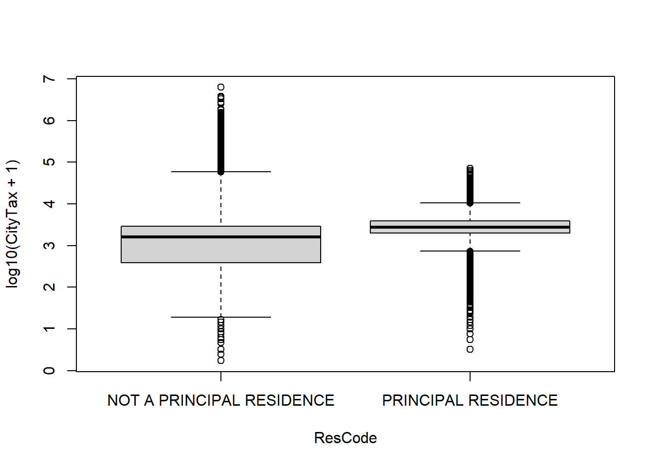
)summarize: now 29 rows and 6 columns, ungrouped- Make boxplots showing
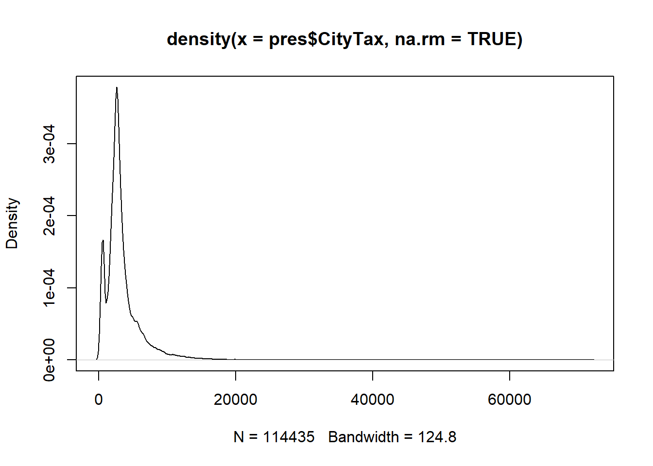
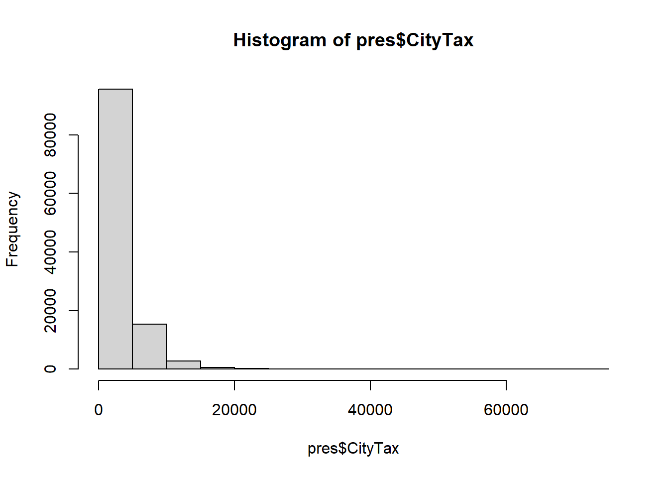
CityTax(y-variable) by whether the property is a principal residence (x = ResCode) or not. You will need to trim some leading/trailing white space fromResCode.
tax = tax %>%
  mutate(ResCode = str_trim(ResCode))
# Using ggplot2
qplot(y = CityTax, x = ResCode, data = tax, geom = "boxplot")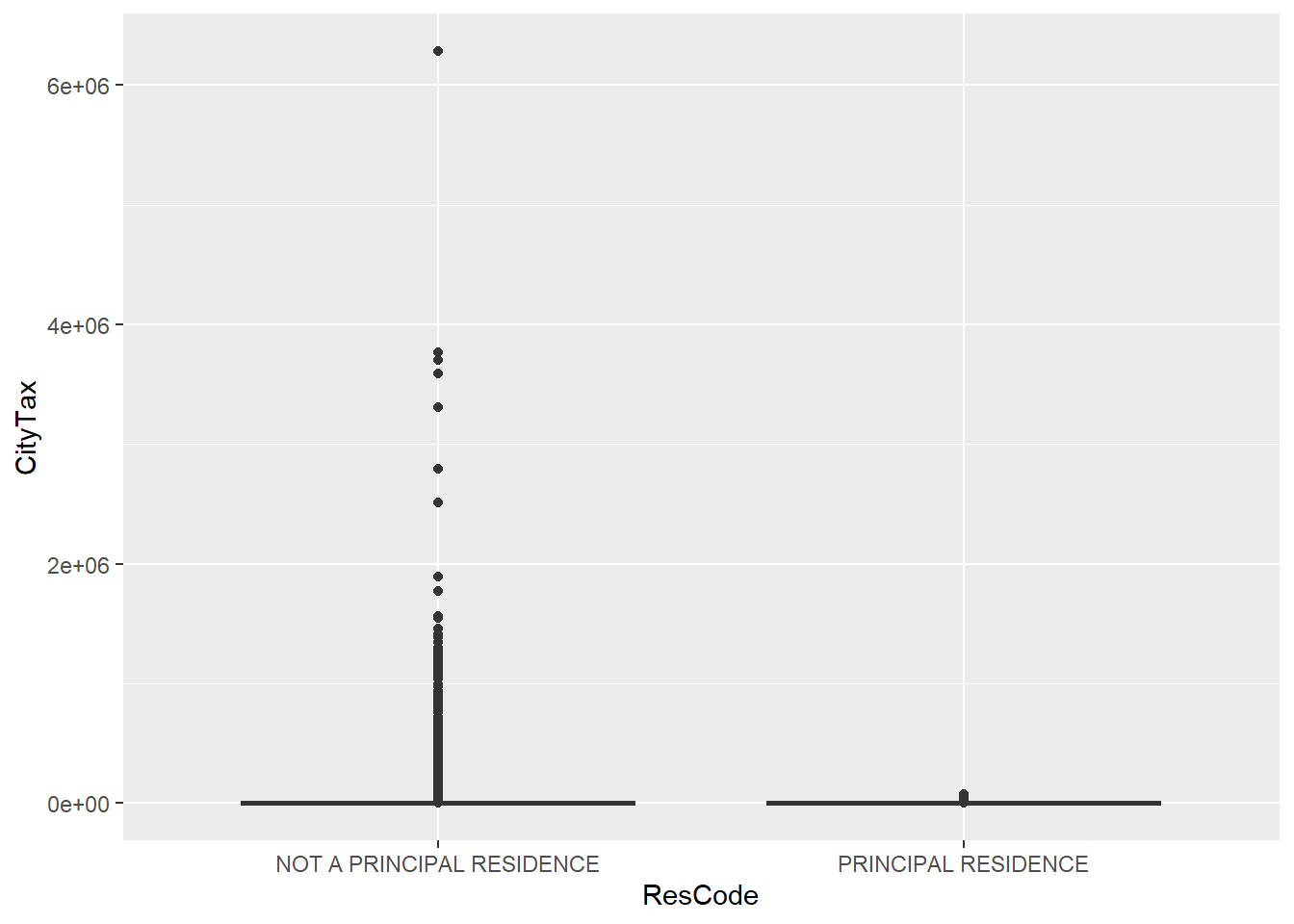
#CityTax is highly right skewed. The log transform makes it more symmetric
qplot(y = log10(CityTax + 1), x = ResCode, data = tax, geom = "boxplot")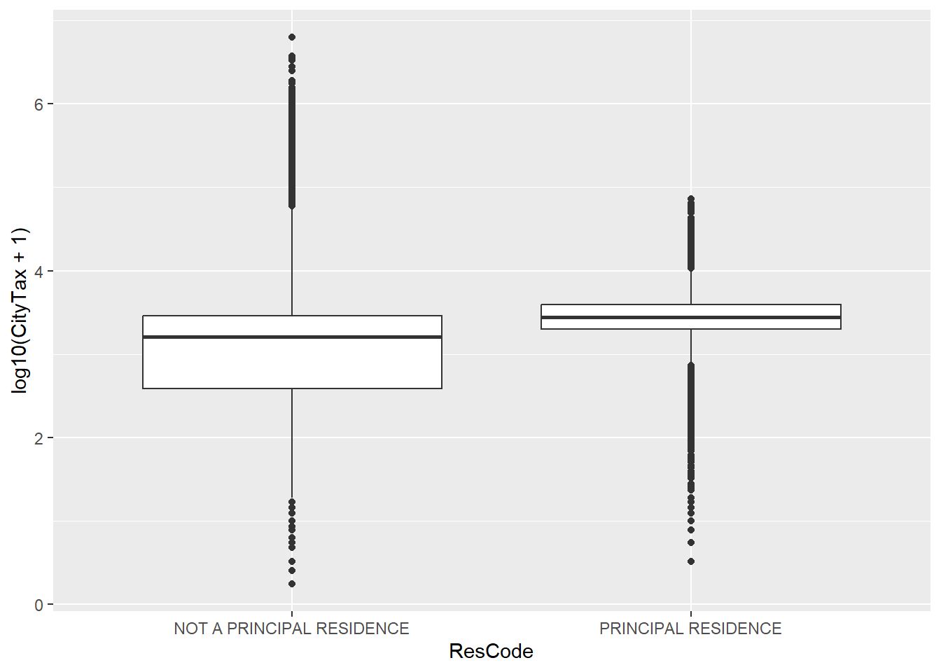
 11. Subset the data to only retain those houses that are principal residences. Which command subsets rows? Filter or select?
a. How many such houses are there?
11. Subset the data to only retain those houses that are principal residences. Which command subsets rows? Filter or select?
a. How many such houses are there?
filter: removed 123,029 rows (52%), 114,934 rows remainingfilter: removed 123,029 rows (52%), 114,934 rows remaining[1] 114934 16b. Describe the distribution of property taxes on these residences. Use `hist`/`qplot` with certain breaks or `plot(density(variable))`.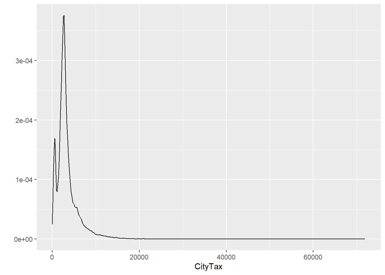
`stat_bin()` using `bins = 30`. Pick better value with `binwidth`.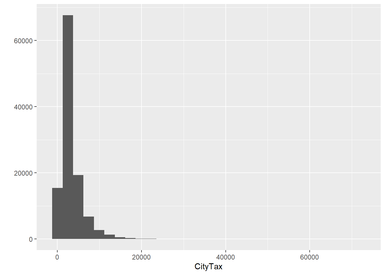
 12. Make an object called
 health.sal using the salaries data set, with only agencies (JobTitle) of those with “fire” (anywhere in the job title), if any, in the name remember fixed("string_match", ignore_case = TRUE) will ignore cases.
sal = read_csv("./data/Baltimore_City_Employee_Salaries_FY2015.csv")
health.sal = sal %>%
  filter(str_detect(JobTitle,
fixed("fire", ignore_case = TRUE)))- Make a data set called
transwhich contains only agencies that contain “TRANS”.
filter: removed 13,982 rows (>99%), 35 rows remaining- What is/are the profession(s) of people who have “abra” in their name for Baltimore’s Salaries? Case should be ignored.
filter: removed 14,005 rows (>99%), 12 rows remaining# A tibble: 12 × 7
name JobTitle AgencyID Agency HireDate AnnualSalary GrossPay
<chr> <chr> <chr> <chr> <chr> <chr> <chr>
1 Abraham,Donta D LABORER (H… B70357 DPW-S… 10/16/2… $30721.00 $32793.…
2 Abraham,Santhosh ACCOUNTANT… A50100 DPW-W… 12/31/2… $49573.00 $49104.…
3 Abraham,Sharon M HOUSING IN… A06043 Housi… 12/15/1… $50365.00 $50804.…
4 Abrahams,Brandon A POLICE OFF… A99416 Polic… 01/20/2… $46199.00 $18387.…
5 Abrams,Maria OFFICE SER… A29008 State… 09/19/2… $35691.00 $34970.…
6 Abrams,Maxine COLLECTION… A14003 FIN-C… 08/26/2… $37359.00 $37768.…
7 Abrams,Terry RECREATION… P04001 R&P-R… 06/19/2… $20800.00 $1690.00
8 Bey,Abraham PROCUREMEN… A17001 FIN-P… 04/23/2… $69600.00 $69763.…
9 Elgamil,Abraham D AUDITOR SU… A24001 COMP-… 01/31/1… $94400.00 $95791.…
10 Gatto,Abraham M POLICE OFF… A99200 Polic… 12/12/2… $66086.00 $73651.…
11 Schwartz,Abraham M GENERAL CO… A54005 FPR A… 07/26/1… $110400.00 $111408…
12 Velez,Abraham L POLICE OFF… A99036 Polic… 10/24/2… $70282.00 $112957…- What does the distribution of annual salaries look like? (use
hist, 20 breaks) What is the IQR? Hint: first convert to numeric. Trystr_replace, but remember$is “special” and you needfixed()around it.
sal = sal %>% mutate(AnnualSalary = str_replace(AnnualSalary, fixed("$"), ""))
sal = sal %>% mutate(AnnualSalary = as.numeric(AnnualSalary))
#ggplot
qplot(x = AnnualSalary, data = sal, geom = "histogram", bins = 20)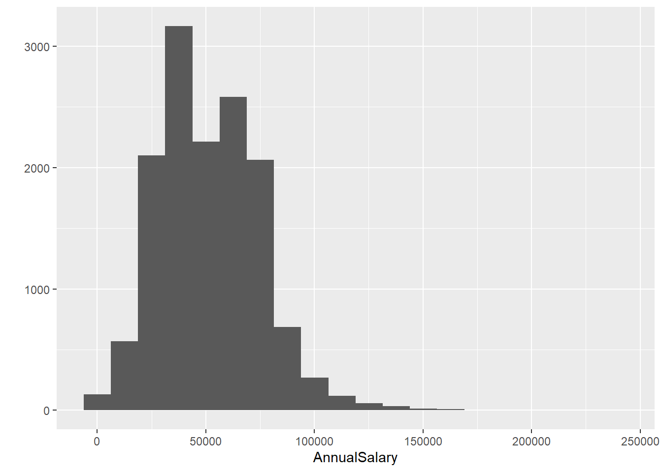
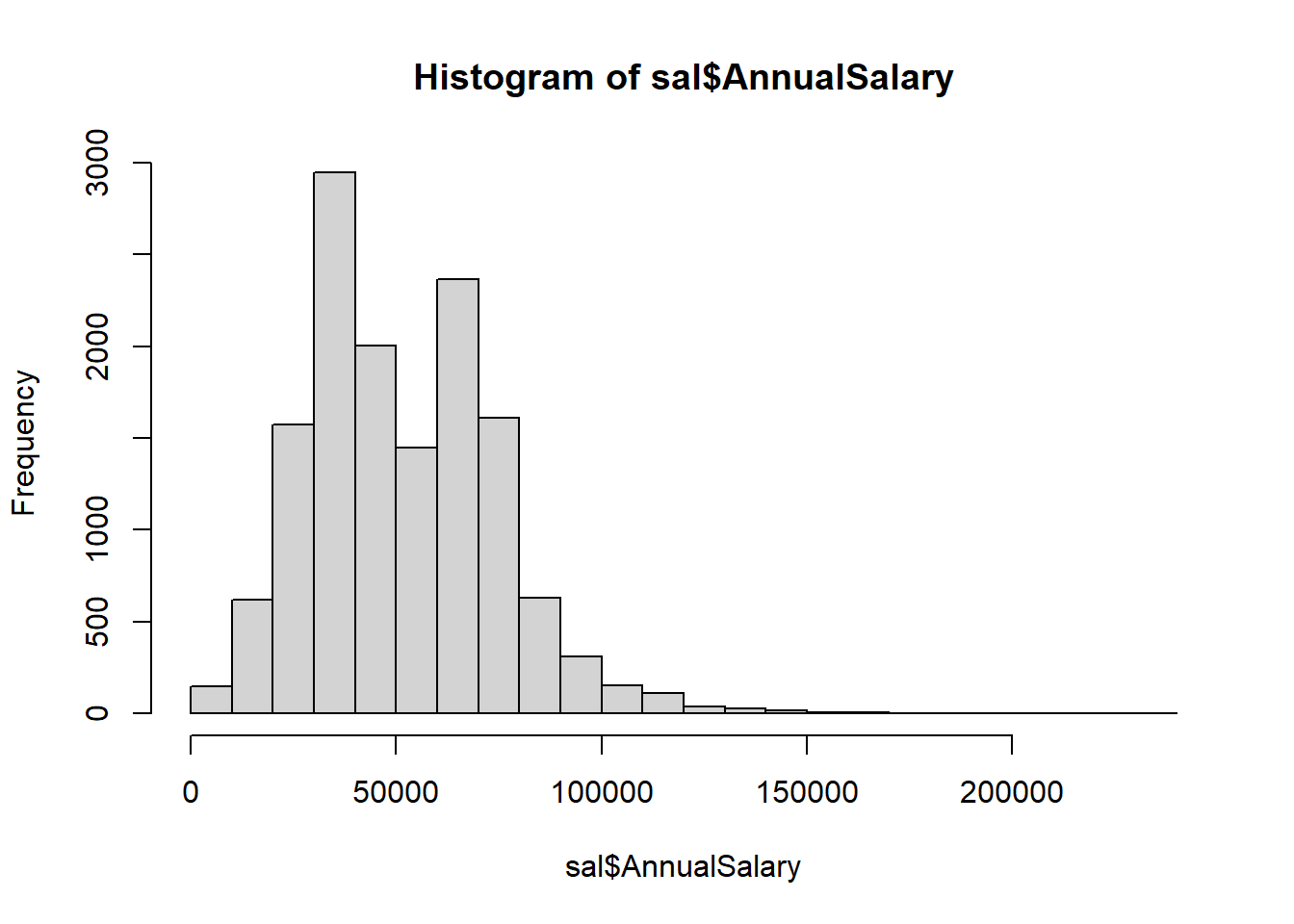
    0%    25%    50%    75%   100%
900 33354 48126 68112 238772 - Convert
HireDateto theDateclass - plot Annual Salary vs Hire Date. UseAnnualSalary ~ HireDatewith adata = salargument in plot or usex,ynotation inscatter.smooth. Use thelubridatepackage. Is itmdy(date)ordmy(date)for this data - look atHireDate.
sal = sal %>% mutate(HireDate = lubridate::mdy(HireDate))

q = qplot(y = AnnualSalary, x = HireDate,
      data = sal, geom = "point")
q + geom_smooth(colour = "red", se = FALSE)
`geom_smooth()` using method = 'gam' and formula = 'y ~ s(x, bs =
"cs")'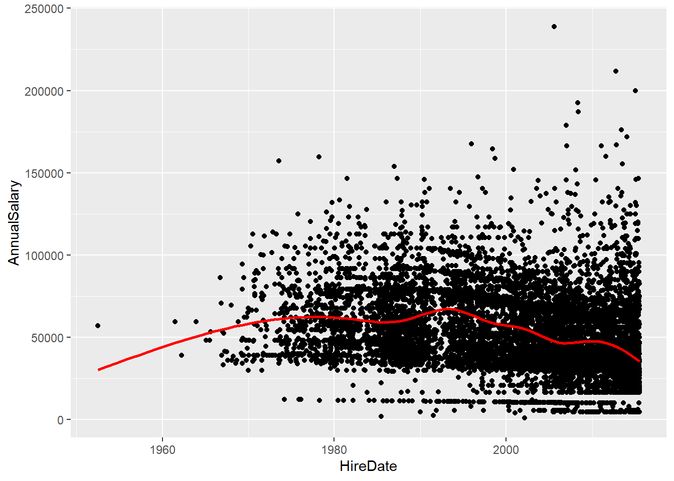
# base R
# plot(AnnualSalary ~ HireDate, data = sal)
# scatter.smooth(sal$AnnualSalary, x = sal$HireDate, col = "red")- Create a smaller dataset that only includes the Police Department, Fire Department and Sheriff’s Office. Use the
Agencyvariable with string matching. Call thisemer. How many employees are in this new dataset?
filter: removed 9,095 rows (65%), 4,922 rows remainingemer = sal %>% filter(
str_detect(Agency, "Sheriff's Office") |
str_detect(Agency, "Police Department") |
str_detect(Agency, "Fire Department")
)filter: removed 9,095 rows (65%), 4,922 rows remaining- Create a variable called
deptin theemerdata set,dept = str_extract(Agency, ".*(ment|ice)"). E.g. we want to extract all characters up until ment or ice (we can group in regex using parentheses) and then discard the rest. Replot annual salary versus hire date and color by dept (not yet - using ggplot). Use the argumentcol = factor(dept)inplot.
emer = emer %>%
mutate(
dept = str_extract(Agency, ".*(ment|ice)")
)
# Replot annual salary versus hire date, color by dept (not yet - using ggplot)
ggplot(aes(x = HireDate, y = AnnualSalary,
colour = dept), data = emer) +
geom_point() + theme(legend.position = c(0.5, 0.8))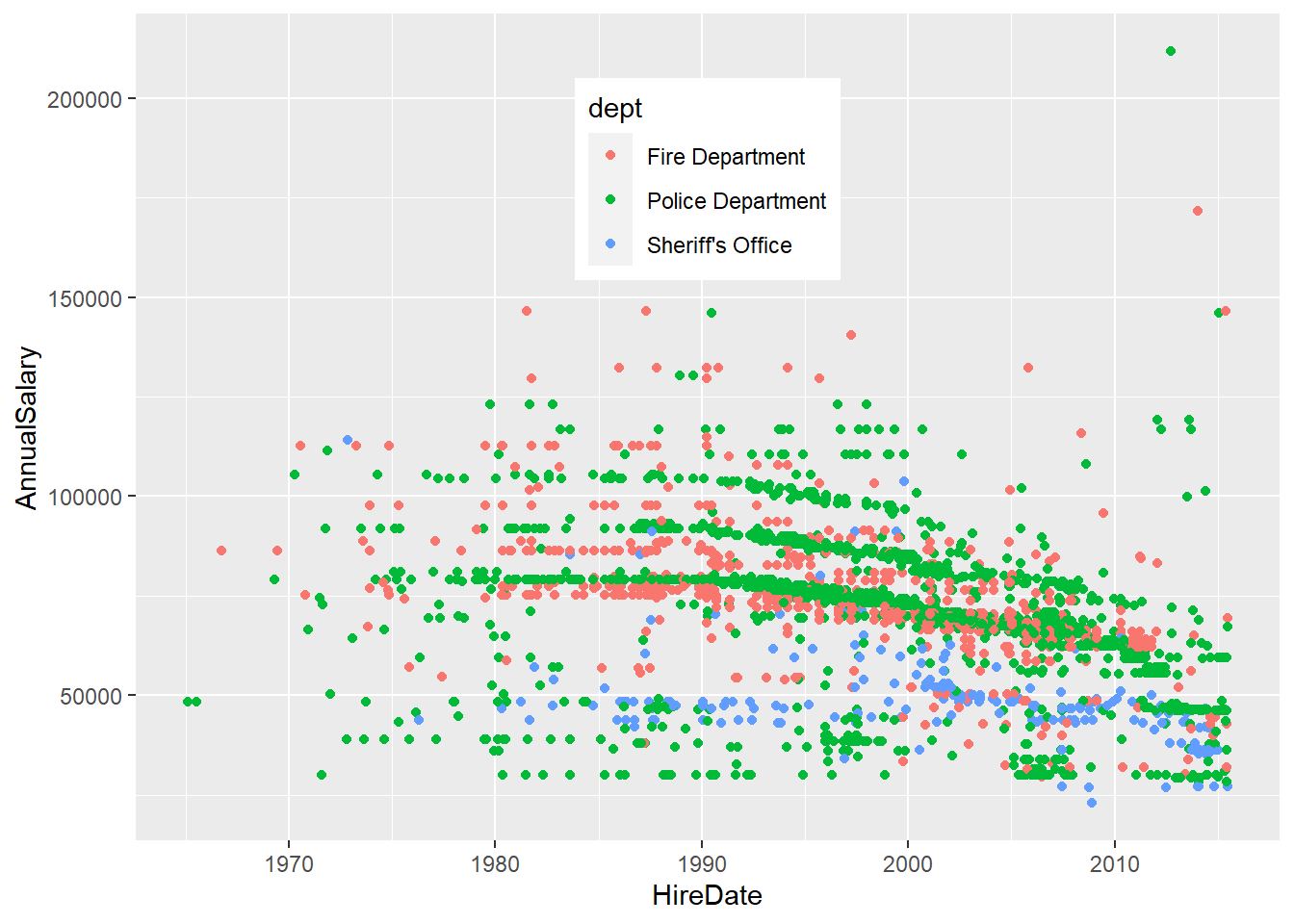 19. (Bonus). Convert the ‘LotSize’ variable to a numeric square feet variable in the
 tax data set. Some tips: a) 1 acre = 43560 square feet b) The hyphens represent a decimals. (This will take a lot of searching to find all the string changes needed before you can convert to numeric.)
First lets take care of acres
[1] 1 2 9 10 11 15[1] "0.020 ACRES" "0.020 ACRES" "0.020 ACRES" "0.020 ACRES" "0.020 ACRES"
[6] "0.020 ACRES"acre = tax$LotSize[aIndex] # temporary variable
## find and replace character strings
acre = str_replace_all(acre, " AC.*","")
acre = str_replace_all(acre, " %","")
table(!is.na(as.numeric(acre)))
FALSE  TRUE
237 18328 [1] "2-158" "O.084" "1-87" "1-85"
[5] "1-8" "1-778" "2-423" "1-791"
[9] "1-81" "O.018" "IMP ONLY 0.190" "26,140"
[13] "8.OOO" "IMP.ONLY 3.615" "2-688" "1.914ACRES"
[17] "2-364" "3-67" "3-46" "3-4"
[21] "2-617" "2-617" "2-617" "4-40"
[25] "3-94" "2-456" "2-486" "2-24"
[29] "1-36" "21-8X5.5" "3-14" "1-566"
[33] "O-70" "16-509" "2-36" "5-25"
[37] "1-005" "0.045ACRES" "0.039ACRES" "0.029ACRES"
[41] "0.029ACRES" "0.041ACRES" "0.048ACRES" "0.053ACRES"
[45] "O.147" "O-602" "O-3567" "28-90"
[49] "4-3165" "1-379" ## lets clean the rest
acre = str_replace_all(acre, "-",".") # hyphen instead of decimal
head(acre[is.na(as.numeric(acre))])[1] "O.084" "O.018" "IMP ONLY 0.190" "26,140"
[5] "8.OOO" "IMP.ONLY 3.615"
FALSE  TRUE
96 18469 [1] "O.084" "O.018" "IMP ONLY 0.190" "26,140"
[5] "8.OOO" "IMP.ONLY 3.615"# take care of individual mistakes
acre = str_replace_all(acre, "O","0") # 0 vs O
acre = str_replace_all(acre, "Q","") # Q, oops
acre = str_replace_all(acre, ",.",".") # extra ,
acre = str_replace_all(acre, ",","") # extra ,
acre = str_replace_all(acre, "L","0") # leading L
acre = str_replace_all(acre, "-",".") # hyphen to period
acre[is.na(as.numeric(acre))][1] "IMP 0N0Y 0.190" "IMP.0N0Y 3.615" "21.8X5.5" [1] 3Now let’s convert all of the square feet variables
library(purrr)
fIndex = which(str_detect(tax$LotSize, "X"))

ft = tax$LotSize[fIndex]

ft = str_replace_all(ft, fixed("&"), "-")
ft = str_replace_all(ft, "IMP ONLY ", "")
ft = str_replace_all(ft, "`","1")

ft= map_chr(str_split(ft, " "), first)

## now get the widths and lengths
width = map_chr(str_split(ft,"X"), first)
length = map_chr(str_split(ft,"X"), nth, 2)

## width
widthFeet = as.numeric(map_chr(str_split(width, "-"), first))
widthInch = as.numeric(map_chr(str_split(width, "-"),nth,2))/12
widthInch[is.na(widthInch)] = 0 # when no inches present
totalWidth = widthFeet + widthInch # add together

# length
lengthFeet = as.numeric(map_chr(str_split(length, "-"),first))
lengthInch = as.numeric(map_chr(str_split(length, "-",2),nth,2))/12

lengthInch[is.na(lengthInch)] = 0 # when no inches present
totalLength = lengthFeet + lengthInch

# combine together for square feet
sqrtFt = totalWidth*totalLength
ft[is.na(sqrtFt)] # what is left?
[1] "161X" "11XX0" "M2X169-9"
[4] "Q8X120" "37-1X-60-10X57-11" "POINT"
[7] "22-11" "ASSESS" "ASSESSCTY56-2X1-1"
[10] "ASSESSCTY53-2X1-1" "O-7X125" "O-3X125"
[13] "X134" "{1-4X128-6" "12-3XX4-2"
[16] "13XX5" "F7-10X80" "N1-8X92-6"
[19] "POINTX100-5X10" "]7X100" "16-11XX5"
[22] "Q5X119" And now we combine everything together:
[1] 0.935456352458# already in square feet, easy!!
sIndex=which(str_detect(tax$LotSize, "FT") | str_detect(tax$LotSize, "S.*F."))
sf = tax$LotSize[sIndex] # subset temporary variable
sqft2 = map_chr(str_split(sf,"( |SQ|SF)"),first)
sqft2 = as.numeric(str_replace_all(sqft2, ",", "")) # remove , and convert
tax$sqft[sIndex] = sqft2
table(is.na(tax$sqft))
 FALSE   TRUE
237771 192 [1] "IMPROVEMENTS ONLY" "0.067" "0.858"
[4] "161X 137" "IMP ONLY" "0.036 ARES"
[7] "11XX0" "IMPROVEMENT ONLY" "IMPROVEMENT ONLY"
[10] "IMPROVEMENT ONLY" "IMPROVEMENT ONLY" "IMPROVEMENT ONLY"
[13] "0.033" "IMPROVEMENT ONLY" "IMPROVEMENT ONLY"
[16] "IMP ONLY" "IMP ONLY 0.190 AC" "IMP ONLY"
[19] "AIR RIGHTS" "AIR RIGHTS" "AIR RIGHTS"
[22] "IMP ONLY" "IMP ONLY" "AIR RIGHTS"
[25] "IMP ONLY" "0.013" "IMP ONLY"
[28] "IMP ONLY" "IMP ONLY" "IMP ONLY"
[31] "196552-8" "0.040" "IMP.ONLY 3.615 AC"
[34] "M2X169-9" "Q8X120" "IMP ONLY"
[37] "IMP ONLY" "IMPROVEMENTS ONLY" "IMPROVEMENTS ONLY"
[40] "IMPROVEMENTS ONLY" "0.016" NA
[43] "0.230" "0.026" "\\560 S.F."
[46] "1233.04" "IMP ONLY" "0.649"
[49] "ASSESSMENT ONLY" "24179D096" "IMPROVEMENT ONLY"
[52] "20080211" NA "IMP ONLY"
[55] "0.028" "IMP ONLY" "IMPROVEMENT ONLY"
[58] "2381437.2 CUBIC F" "IMP ONLY" "IMP ONLY"
[61] "IMPROVEMENTS ONLY" "AIR RIGHTS ONLY" "IMP ONLY"
[64] "IMP ONLY" "37-1X-60-10X57-11" "IMPROVEMENT ONLY"
[67] "IMPROVEMENT ONLY" "IMPROVEMENT ONLY" "IMPROVEMENT ONLY"
[70] "IMPROVEMENT ONLY" "IMP ONLY" "IMP ONLY"
[73] "IMP ONLY" "IMP ONLY" "POINT X 57-9"
[76] "IMP ONLY" "AIR RIGHTS" "0.5404%"
[79] "IMPROVEMENT ONLY" "IMP ONLY" "19520819"
[82] NA "0.024" "IMPROVEMENT ONLY"
[85] "IMPROVEMENT ONLY" "68I.0 SQ FT" "11979"
[88] "1159-0 S.F." "IMPROVEMENT ONLY" NA
[91] "IMPROVEMENT ONLY" "0.039" "IMPROVEMENT ONLY"
[94] "IMP ONLY" "IMP ONLY" "IMPROVEMENT ONLY"
[97] "IMP ONLY" "IMP ONLY" "0.681 ARCES"
[100] "7,138 SF" "13,846 SF" "9,745 SF"
[103] "13,772 SF" "17,294 SF" "15,745 SF"
[106] "18, 162 SF" "01185" "AIR RIGHTS"
[109] "AIR RIGHTS" "IMPROVEMENTS ONLY" "22-11 X57"
[112] "0.129%" "0.129%" "0.129%"
[115] "0.129%" "0.129%" "ASSESS CTY 84 S.F"
[118] "IMPROVEMENT ONLY" "ASSESS CTY 50 S.F" "ASSESS CTY 57X1-1"
[121] "IMP ONLY" "ASSESSCTY56-2X1-1" "ASSESSCTY53-2X1-1"
[124] "IMPROVEMENT ONLY" "IMPROVEMENT ONLY" "O-7X125"
[127] "O-3X125" "0.026" "X134"
[130] "{1-4X128-6" NA NA
[133] NA "IMPROVEMENT ONLY" "IMPROVEMENT ONLY"
[136] "12-3XX4-2" "13XX5" "ASSESS CTY"
[139] "IMP ONLY" "IMP ONLY" "IMP ONLY"
[142] "IMP ONLY" "IMPROVEMENTS ONLY" "IMPROVEMENT ONLY"
[145] "0.032" "20050712" "F7-10X80"
[148] "IMP ONLY" "IMP ONLY" "0.033"
[151] "03281969" "IMP.ONLY" "IMP ONLY"
[154] "REAR PART 697 S.F" "IMP ONLY" "IMPROVEMENT ONLY"
[157] "N1-8X92-6" "POINTX100-5X10" "IMPROVEMENTS ONLY"
[160] "]7X100" "07031966" "13O4 SQ FT"
[163] "05081978" "0.030" "IMPROVEMENTS ONLY"
[166] "AIR RIGHTS" "AIR RIGHTS" "IMPROVEMENT ONLY"
[169] "IMPROVEMENT ONLY" "IMPROVEMENT ONLY" "IMPROVEMENT ONLY"
[172] "0.191 ARES" "19815-4" "11`79"
[175] NA NA "IMPROVEMENT ONLY"
[178] "IMP ONLY" "194415" "IMP ONLY"
[181] "IMPROVEMENT ONLY" "IMP ONLY" "120-103"
[184] "IMP ONLY" "IMP. ONLY" "196700"
[187] "IMPROVEMENT ONLY" "16-11XX5" "Q5X119"
[190] "21210" "IMPROVEMENT ONLY" "5306120" There are still many strings that need to be removed before we can convert
16.8 Mainpulating Data
- Read in the Bike_Lanes_Wide.csv dataset and call is
wide.
Rows: 134 Columns: 9
── Column specification ──────────────────────────────────────────────
Delimiter: ","
chr (1): name
dbl (8): BIKE BOULEVARD, BIKE LANE, CONTRAFLOW, SHARED BUS BIKE, SHARROW, SI...

ℹ Use `spec()` to retrieve the full column specification for this data.
ℹ Specify the column types or set `show_col_types = FALSE` to quiet this message.- Reshape
wideusingpivot_longer. Call this datalong. Make the keylanetype, and the valuethe_length. Make sure we gather all columns butname, using-name. Note theNAshere.
pivot_longer: reorganized (BIKE BOULEVARD, BIKE LANE, CONTRAFLOW, SHARED BUS BIKE, SHARROW, …) into (lanetype, the_length) [was 134x9, now 1072x3]# A tibble: 6 × 3
name lanetype the_length
<chr> <chr> <dbl>
1 ALBEMARLE ST BIKE BOULEVARD NA
2 ALBEMARLE ST BIKE LANE NA
3 ALBEMARLE ST CONTRAFLOW NA
4 ALBEMARLE ST SHARED BUS BIKE NA
5 ALBEMARLE ST SHARROW 110.
6 ALBEMARLE ST SIDEPATH NA - Read in the roads and crashes .csv files and call them
roadandcrash.
Rows: 110 Columns: 4
── Column specification ──────────────────────────────────────────────
Delimiter: ","
chr (1): Road
dbl (3): Year, N_Crashes, Volume

ℹ Use `spec()` to retrieve the full column specification for this data.
ℹ Specify the column types or set `show_col_types = FALSE` to quiet this message.Rows: 5 Columns: 3
── Column specification ──────────────────────────────────────────────
Delimiter: ","
chr (2): Road, District
dbl (1): Length
ℹ Use `spec()` to retrieve the full column specification for this data.
ℹ Specify the column types or set `show_col_types = FALSE` to quiet this message.# A tibble: 6 × 4
Year Road N_Crashes Volume
<dbl> <chr> <dbl> <dbl>
1 1991 Interstate 65 25 40000
2 1992 Interstate 65 37 41000
3 1993 Interstate 65 45 45000
4 1994 Interstate 65 46 45600
5 1995 Interstate 65 46 49000
6 1996 Interstate 65 59 51000# A tibble: 5 × 3
Road District Length
<chr> <chr> <dbl>
1 Interstate 65 Greenfield 262
2 Interstate 70 Vincennes 156
3 US-36 Crawfordsville 139
4 US-40 Greenfield 150
5 US-52 Crawfordsville 172- Replace (using
str_replace) any hyphens (-) with a space incrash$Road. Call this datacrash2. Table theRoadvariable.
Interstate 275  Interstate 65  Interstate 70          US 36          US 40
22 22 22 22 22 - How many observations are in each dataset?
[1] 110 4[1] 5 3- Separate the
Roadcolumn (usingseparate) into (typeandnumber) incrash2. Reassign this tocrash2. Tablecrash2$type. Then create a new variable calling itroad_hyphenusing theunitefunction. Unite thetypeandnumbercolumns using a hyphen (-) and then tableroad_hyphen.
Interstate         US
        66         44
Interstate-275  Interstate-65  Interstate-70          US-36          US-40
22 22 22 22 22 - Which and how many years were data collected in the
crashdataset?
 [1] 1991 1992 1993 1994 1995 1996 1997 1998 1999 2000 2001 2002 2003 2004 2005
[16] 2006 2007 2008 2009 2010 2011 2012[1] 22- Read in the dataset Bike_Lanes.csv and call it
bike.
- Keep rows where the record is not missing
typeand not missingnameand re-assign the output tobike.
filter: removed 21 rows (1%), 1,610 rows remaining- Summarize and group the data by grouping
nameandtype(i.e for each type within each name) and take thesumof thelength(reassign the sum of the lengths to thelengthvariable). Call this data setsub.
summarize: now 162 rows and 3 columns, one group variable remaining (name)- Reshape
subusingpivot_wider. Spread the data where the key istypeand we want the value in the new columns to belength- the bike lane length. Call thiswide2. Look at the column names ofwide2- what are they? (they also have spaces).
pivot_wider: reorganized (type, length) into (SHARROW, SIGNED ROUTE, BIKE LANE, CONTRAFLOW, SHARED BUS BIKE, …) [was 162x3, now 132x8]Look at the column names of wide. What are they? (they also have spaces)
[1] "name"            "SHARROW"         "SIGNED ROUTE"    "BIKE LANE"
[5] "CONTRAFLOW" "SHARED BUS BIKE" "SIDEPATH" "BIKE BOULEVARD" - Join data in the crash and road datasets to retain only complete data, (using an inner join) e.g. those observations with road lengths and districts. Merge without using
byargument, then merge usingby = "Road". call the output merged. How many observations are there?
Joining with `by = join_by(Road)`
inner_join: added 2 columns (District, Length)
> rows only in x (22)
> rows only in y ( 1)
> matched rows 88
> ====
> rows total 88inner_join: added 2 columns (District, Length)
> rows only in x (22)
> rows only in y ( 1)
> matched rows 88
> ====
> rows total 88[1] 88 6- Join data using a
full_join. Call the outputfull. How many observations are there?
Joining with `by = join_by(Road)`
full_join: added 2 columns (District, Length)
> rows only in x 22
> rows only in y 1
> matched rows 88
> =====
> rows total 111full_join: added 2 columns (District, Length)
> rows only in x 22
> rows only in y 1
> matched rows 88
> =====
> rows total 111[1] 111- Do a left join of the
roadandcrash. ORDER matters here! How many observations are there?
Joining with `by = join_by(Road)`
left_join: added 3 columns (Year, N_Crashes, Volume)
> rows only in x 1
> rows only in y (22)
> matched rows 88 (includes duplicates)
> ====
> rows total 89left_join: added 3 columns (Year, N_Crashes, Volume)
> rows only in x 1
> rows only in y (22)
> matched rows 88 (includes duplicates)
> ====
> rows total 89[1] 89- Repeat above with a
right_joinwith the same order of the arguments. How many observations are there?
Joining with `by = join_by(Road)`
right_join: added 3 columns (Year, N_Crashes, Volume)
> rows only in x ( 1)
> rows only in y 22
> matched rows 88
> =====
> rows total 110right_join: added 3 columns (Year, N_Crashes, Volume)
> rows only in x ( 1)
> rows only in y 22
> matched rows 88
> =====
> rows total 110[1] 11016.9 Data Visualization
library(readr)
library(ggplot2)
library(tidyr)
library(dplyr)
library(lubridate)
library(stringr)

circ = read_csv("./data/Charm_City_Circulator_Ridership.csv")

# covert dates
circ = mutate(circ, date = mdy(date))
# change colnames for reshaping
colnames(circ) =  colnames(circ) %>%
  str_replace("Board", ".Board") %>%
  str_replace("Alight", ".Alight") %>%
  str_replace("Average", ".Average")

# make long
long = gather(circ, "var", "number",
              starts_with("orange"),
              starts_with("purple"), starts_with("green"),
              starts_with("banner"))
# separate
long = separate(long, var, into = c("route", "type"),
    sep = "[.]")

## take just average ridership per day
avg = filter(long, type == "Average")
avg = filter(avg, !is.na(number))

# separate
type_wide = spread(long, type, value = number)
head(type_wide)
# A tibble: 6 × 7
day date daily route Alightings Average Boardings
<chr> <date> <dbl> <chr> <dbl> <dbl> <dbl>
1 Friday 2010-01-15 1644 banner NA NA NA
2 Friday 2010-01-15 1644 green NA NA NA
3 Friday 2010-01-15 1644 orange 1643 1644 1645
4 Friday 2010-01-15 1644 purple NA NA NA
5 Friday 2010-01-22 1394. banner NA NA NA
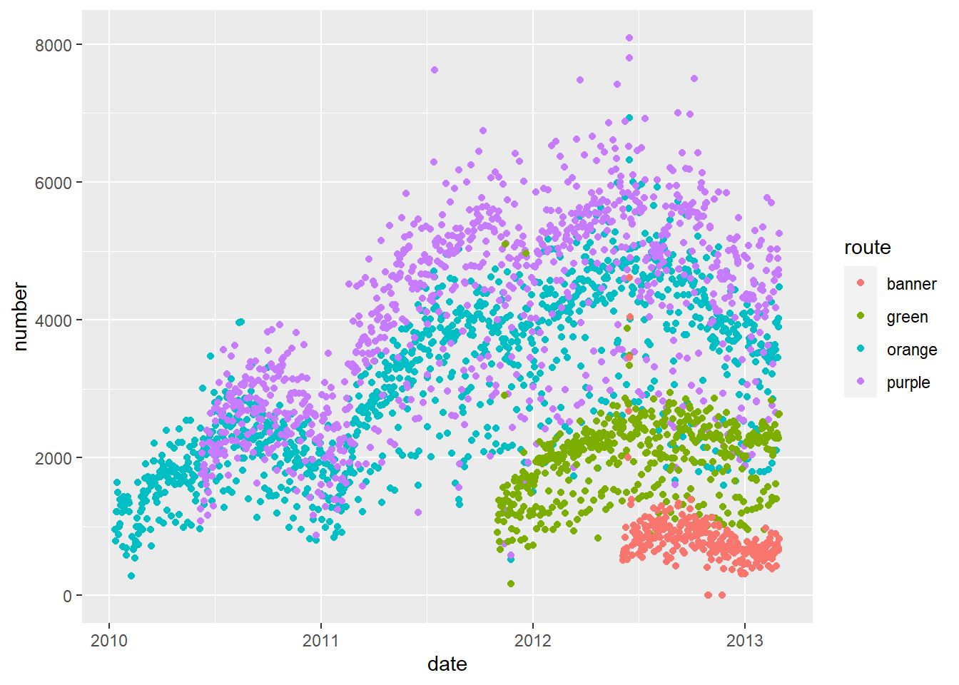
6 Friday 2010-01-22 1394. green NA NA NA- Plot average ridership (
avgdata set) bydateusing a scatterplot.- Color the points by route (
orange,purple,green,banner)
- Color the points by route (
 b. Add black smoothed curves for each route
qplot(x = date, y = number, data = avg, colour = route) +
  geom_smooth(aes(group = route), colour= "black") #change the smoothed line to black so it is more visible
`geom_smooth()` using method = 'gam' and formula = 'y ~ s(x, bs =
"cs")'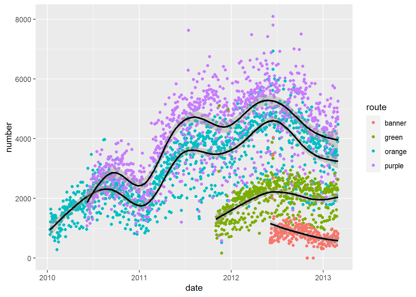 c. Color the points by day of the week
# qplot(x = date, y = number, data = avg, colour = day)
# This way the legend appears on order for days of the week
avg = avg %>% mutate(dayFactor = factor(day, levels = c("Monday", "Tuesday", "Wednesday", "Thursday", "Friday", "Saturday", "Sunday")))
g = ggplot(avg, aes(x = date, y = number, color = dayFactor))
g + geom_point()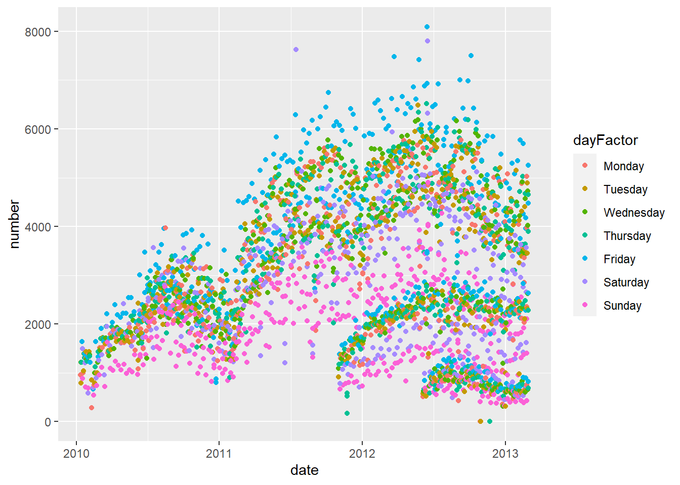 2. Replot 1a where the colors of the points are the name of the
 route (with banner –> blue)
pal = c("blue", "darkgreen","orange","purple")
# qplot(x = date, y = number, data = avg, colour = route) +
# scale_colour_manual(values = pal)
g = ggplot(avg, aes(x = date, y = number, color = route))
g + geom_point() + scale_colour_manual(values = pal)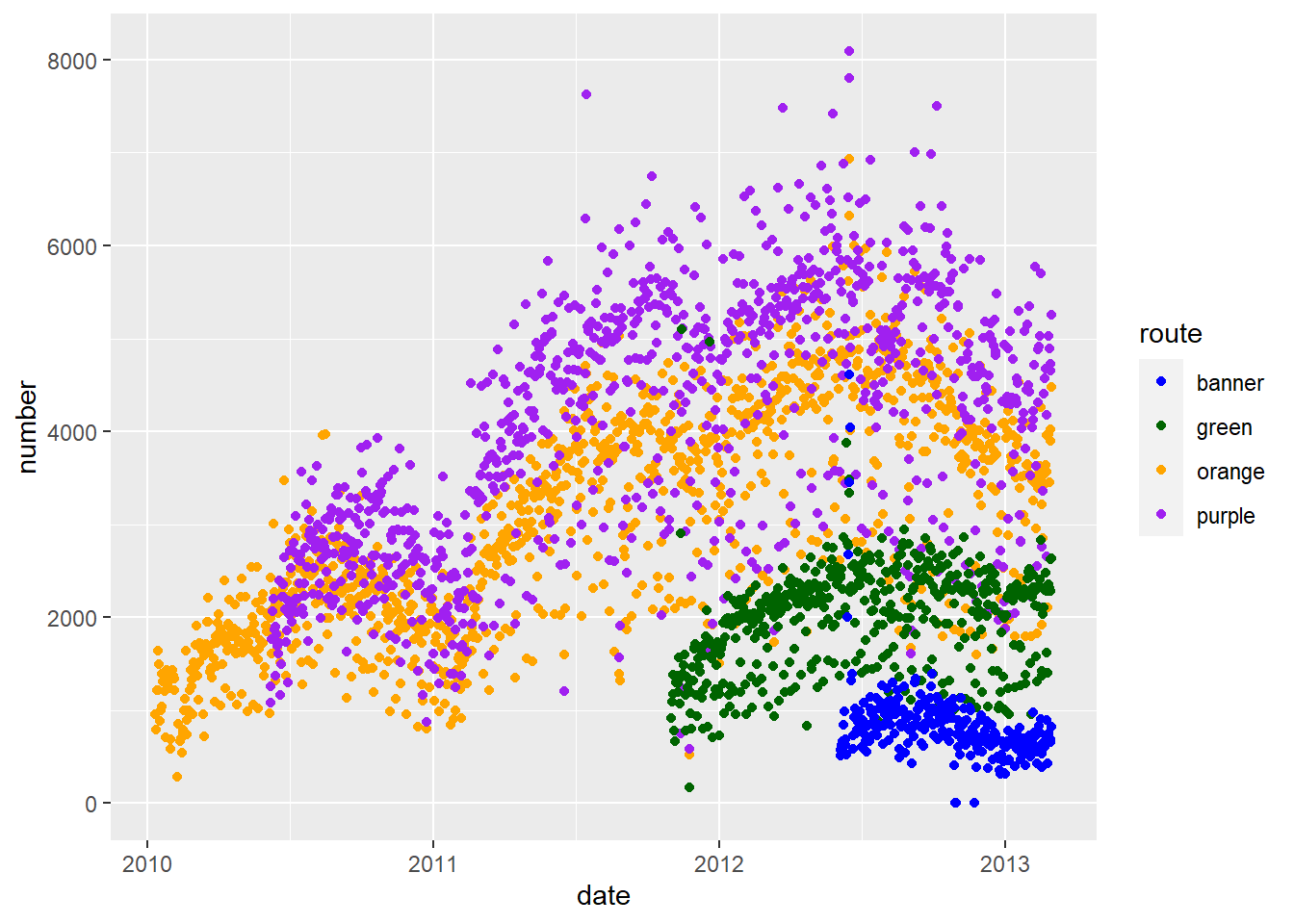 3. Plot average ridership by date with one panel per
 route
g = ggplot(avg, aes(x = date, y = number, color = route))
g + geom_point() +
facet_wrap( ~ route) +
scale_colour_manual(values=pal)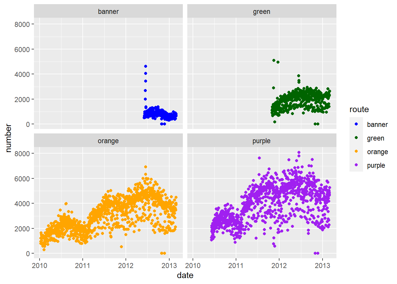 4. Plot average ridership by date with separate panels by
 day of the week, colored by route.
ggplot(aes(x = date, y = number, colour = route), data= avg) +
geom_point() +
facet_wrap( ~dayFactor) + scale_colour_manual(values=pal)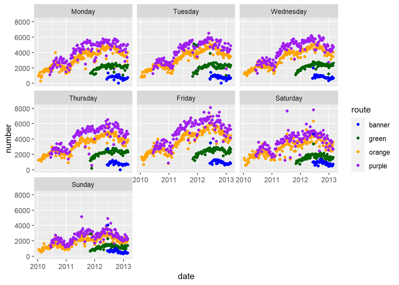 5. Plot average ridership (
avg) by date, colored by route (same as 1a). (do not take an average, use the average column for each route). Make the x-label "Year". Make the y-label "Number of People". Use the black and white theme theme_bw(). Change the text_size to (text = element_text(size = 20)) in theme.
first_plot = ggplot(avg, aes(x = date, y = number, color = route)) +
geom_point() + scale_colour_manual(values=pal)
first_plot +
xlab("Year") + ylab("Number of People") + theme_bw() +
theme(text = element_text(size = 20))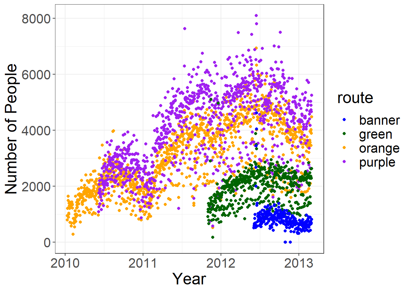 6. Plot average ridership on the
 orange route versus date as a solid line, and add dashed “error” lines based on the boardings and alightings. The line colors should be orange. (hint linetype is an aesthetic for lines - see also scale_linetype and scale_linetype_manual. Use Alightings = "dashed", Boardings = "dashed", Average = "solid")
filter: removed 10,314 rows (75%), 3,438 rows remainingggplot(orange, aes(x = date, y = number)) +
geom_line(aes(linetype = type), colour = "orange") +
scale_linetype_manual(
values = c(Alightings = "dashed",
Boardings = "dashed",
Average = "solid"))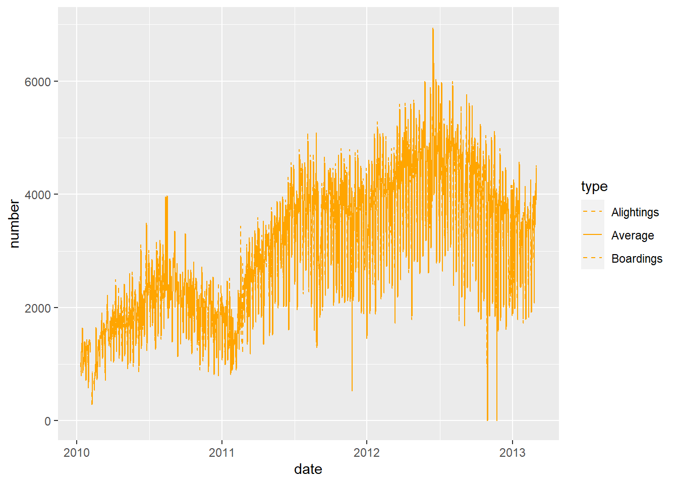 The following zooms in on a section of the plot, so you can actually see the three lines
16.10 Statistical Analysis
library(readr)
library(dplyr)
mort = read_csv("./data/indicatordeadkids35.csv")
mort = mort %>%
dplyr::rename(country = "...1")- Compute the correlation between the
1980,1990,2000, and2010mortality data. No need to save this in an object. Just display the result to the screen. Note anyNAs. Then compute usinguse = "complete.obs".
               1980           1990           2000 2010
1980 1.000000000000 0.960153953723 0.888841117492   NA
1990 0.960153953723 1.000000000000 0.961384203917   NA
2000 0.888841117492 0.961384203917 1.000000000000   NA
2010 NA NA NA 1 1980 1990 2000 2010
1980 1.000000000000 0.959684628292 0.887743334542 0.846828397953
1990 0.959684628292 1.000000000000 0.961026893827 0.924719217724
2000 0.887743334542 0.961026893827 1.000000000000 0.986234456933
2010 0.846828397953 0.924719217724 0.986234456933 1.000000000000 1980 1990 2000 2010
1980 1.000000000000 0.960153953723 0.888841117492 NA
1990 0.960153953723 1.000000000000 0.961384203917 NA
2000 0.888841117492 0.961384203917 1.000000000000 NA
2010 NA NA NA 1 1980 1990 2000 2010
1980 1.000000000000 0.960153953723 0.888841117492 NA
1990 0.960153953723 1.000000000000 0.961384203917 NA
2000 0.888841117492 0.961384203917 1.000000000000 NA
2010 NA NA NA 1- Compute the correlation between the
Myanmar,China, andUnited Statesmortality data. Store this correlation matrix in an object calledcountry_cor
- Compute the correlation between the
mort_subs = mort %>%
  filter(country %in% c("China", "Myanmar","United States")) %>%
  arrange(country)
filter: removed 194 rows (98%), 3 rows remaininglong = mort_subs %>%
pivot_longer( -country, names_to = "year", values_to = "death") %>%
filter(!is.na(death))pivot_longer: reorganized (1760, 1761, 1762, 1763, 1764, …) into (year, death) [was 3x255, now 762x3]filter: removed 120 rows (16%), 642 rows remainingpivot_wider: reorganized (country, death) into (China, Myanmar, United States) [was 642x3, now 214x4] Myanmar China United States
Myanmar 1.000000000000 0.974364554315 0.629262462521
China 0.974364554315 1.000000000000 0.690926321344
United States 0.629262462521 0.690926321344 1.000000000000#alternatively
mort_subs = mort %>%
filter(country %in% c("China", "Myanmar","United States")) %>%
dplyr::select(-country)filter: removed 194 rows (98%), 3 rows remainingb. Extract the Myanmar-US correlation from the correlation matrix.Run the following to see that the order is China, Myanmar, US:
[1] 0.629262462521Extract the Myanmar-US correlation.
[1] 0.629262462521- Is there a difference between mortality information from
1990and2000? Run a t-test and a Wilcoxon rank sum test to assess this. Hint: to extract the column of information for1990, usemort$"1990"
Paired t-test
data: mort$"1990" and mort$"2000"
t = 10.02534013, df = 196, p-value < 2.220446e-16
alternative hypothesis: true mean difference is not equal to 0
95 percent confidence interval:
0.127776911751 0.190359276239
sample estimates:
mean difference
0.159068093995
Wilcoxon signed rank test with continuity correction
data: mort$`1990` and mort$`2000`
V = 17997, p-value < 2.220446e-16
alternative hypothesis: true location shift is not equal to 0- Using the cars dataset, fit a linear regression model with vehicle cost (
VehBCost) as the outcome and vehicle age (VehicleAge) and whether it’s an online sale (IsOnlineSale) as predictors as well as their interaction. Save the model fit in an object calledlmfit_carsand display the summary table.
cars = read_csv("./data/kaggleCarAuction.csv",
col_types = cols(VehBCost = col_double()))
lmfit_cars = lm(VehBCost ~ VehicleAge + IsOnlineSale + VehicleAge:IsOnlineSale,
data = cars)# A tibble: 4 × 5
term estimate std.error statistic p.value
<chr> <dbl> <dbl> <dbl> <dbl>
1 (Intercept) 8063. 16.6 486. 0
2 VehicleAge -321. 3.67 -87.4 0
3 IsOnlineSale 514. 108. 4.77 0.00000180
4 VehicleAge:IsOnlineSale -55.4 25.6 -2.17 0.0303 - Create a variable called
expensivein thecarsdata that indicates if the vehicle cost is over$10,000. Use a chi-squared test to assess if there is a relationship between a car being expensive and it being labeled as a “bad buy” (IsBadBuy).
cars = cars %>%
mutate(expensive = VehBCost > 10000)
tab = table(cars$expensive, cars$IsBadBuy)
chisq.test(tab)
Pearson's Chi-squared test with Yates' continuity correction
data: tab
X-squared = 1.815247312, df = 1, p-value = 0.177880045- Fit a logistic regression model where the outcome is “bad buy” status and predictors are the
expensivestatus and vehicle age (VehicleAge). Save the model fit in an object calledlogfit_carsand display the summary table. Use summary ortidy(logfit_cars, conf.int = TRUE, exponentiate = TRUE)ortidy(logfit_cars, conf.int = TRUE, exponentiate = FALSE)for log odds ratios
logfit_cars = glm(IsBadBuy ~ expensive + VehicleAge, data = cars, family = binomial)
#logfit_cars = glm(IsBadBuy ~ expensive + VehicleAge, data = cars, family = binomial())
#logfit_cars = glm(IsBadBuy ~ expensive + VehicleAge, data = cars, family = "binomial")
summary(logfit_cars)
Call:
glm(formula = IsBadBuy ~ expensive + VehicleAge, family = binomial,
data = cars)
Coefficients:
Estimate Std. Error z value Pr(>|z|)
(Intercept) -3.24948976307 0.03324440927 -97.74545 < 2e-16 ***
expensiveTRUE -0.08038741797 0.06069562592 -1.32444 0.18536
VehicleAge 0.28660451302 0.00647588104 44.25722 < 2e-16 ***
---
Signif. codes: 0 '***' 0.001 '**' 0.01 '*' 0.05 '.' 0.1 ' ' 1
(Dispersion parameter for binomial family taken to be 1)
Null deviance: 54421.30728 on 72982 degrees of freedom
Residual deviance: 52441.78751 on 72980 degrees of freedom
AIC: 52447.78751
Number of Fisher Scoring iterations: 5# A tibble: 3 × 7
term estimate std.error statistic p.value conf.low conf.high
<chr> <dbl> <dbl> <dbl> <dbl> <dbl> <dbl>
1 (Intercept) 0.0388 0.0332 -97.7 0 0.0363 0.0414
2 expensiveTRUE 0.923 0.0607 -1.32 0.185 0.818 1.04
3 VehicleAge 1.33 0.00648 44.3 0 1.32 1.35 # A tibble: 3 × 7
term estimate std.error statistic p.value conf.low conf.high
<chr> <dbl> <dbl> <dbl> <dbl> <dbl> <dbl>
1 (Intercept) -3.25 0.0332 -97.7 0 -3.31 -3.18
2 expensiveTRUE -0.0804 0.0607 -1.32 0.185 -0.201 0.0370
3 VehicleAge 0.287 0.00648 44.3 0 0.274 0.299 16.11 Functions
- Write a function,
sqdif, that does the following:- takes two numbers
xandywith default values of 2 and 3. - takes the difference
- squares this difference
- then returns the final value
- checks that
xandyare numeric andstops with an error message otherwise.
- takes two numbers
sqdif = function(x = 2, y = 3) {
if (!is.numeric(x) | !is.numeric(y)){
stop("Both x and y must be numeric")
} else return((x - y)^2)
}
sqdiffunction(x = 2, y = 3) {
if (!is.numeric(x) | !is.numeric(y)){
stop("Both x and y must be numeric")
} else return((x - y)^2)
}[1] 25Error in sqdif("5", 1): Both x and y must be numeric- Try to write a function called
top()that takes amatrixordata.frameand a numbern, and returns the firstnrows and columns, with the default value ofn=5.
[,1] [,2] [,3] [,4] [,5]
[1,] 1 11 21 31 41
[2,] 2 12 22 32 42
[3,] 3 13 23 33 43
[4,] 4 14 24 34 44
[5,] 5 15 25 35 45 [,1] [,2]
[1,] 1 6
[2,] 2 7- Write a function that will calculate a 95% one sample t interval. The results will be stored in a list to be returned containing sample mean and the confidence interval. The input the functions is the numeric vector containing our data. For review, the formula for a 95% one sample t-interval is \(\bar{x} \pm 1.96*s/\sqrt{n}\).
my_t_CI = function(x) {
x_bar = mean(x)
n = length(x)
z = qt(0.975, df = n-1) # approximately 1.96 for large n
CI.lower = x_bar - z*sd(x) / sqrt(n)
CI.upper = x_bar + z*sd(x) / sqrt(n)
return(list(x_bar = x_bar, CI.lower = CI.lower, CI.upper = CI.upper))
}
data_sim = rnorm(100)
my_t_CI(data_sim)$x_bar
[1] 0.0472156866557
$CI.lower
[1] -0.154868109042
$CI.upper
[1] 0.249299482354
One Sample t-test
data: data_sim
t = 0.4636005847, df = 99, p-value = 0.6439516
alternative hypothesis: true mean is not equal to 0
95 percent confidence interval:
-0.154868109042 0.249299482354
sample estimates:
mean of x
0.0472156866557 16.12 Simulations
- Simulate a random sample of size \(n=100\) from
- a normal distribution with mean 0 and variance 1. (see
rnorm)
- a normal distribution with mean 0 and variance 1. (see
[1] 0.24657838830181 -0.28315247004084 0.27358560551538 0.73355368164771
[5] 0.00590490085201 -1.81955582293960b. a normal distribution with mean 1 and variance 1. (see `rnorm`)[1] 0.468497914898 0.720659579491 0.812009696163 3.227644726789 1.094358592940
[6] 1.587670874195c. a uniform distribution over the interval [-2, 2]. (see `runif`)[1] -1.5004615578800 -0.4790567662567 0.8695481279865 -0.0178337078542
[5] 1.8206319734454 -0.0594882853329- Run a simulation experiment to see how the type I error rate behaves for a two sided one sample t-test when the true population follows a Uniform distribution over [-10,10]. Modify the function
t.test.simthat we wrote to run this simulation by- changing our random samples of size
nto come from a uniform distribution over [-10,10] (seerunif). - performing a two sided t-test instead of a one sided t-test.
- performing the test at the 0.01 significance level.
- choosing an appropriate value for the null value in the t-test. Note that the true mean in this case is 0 for a Uniform(-10,10) population.
Try this experiment for
n=10,30,50,100,500. What happens the estimated type I error rate asnchanges? Is the type I error rate maintained for any of these sample sizes?
- changing our random samples of size
t.test.sim = function(n = 30, N = 1000){
reject = logical(N) #Did this sample lead to a rejection of H0?
for (i in 1:N) {
x = runif(n, -10, 10) #generate a sample of size n from Exp(1) distribution
t.test.p.value = t.test(x, mu = 0, alternative = "two.sided")$p.value
reject[i] = (t.test.p.value < 0.01) #Do we reject H0?
}
mean(reject) #estimated type 1 error rate
}
t.test.sim(n = 10)[1] 0.01[1] 0.011[1] 0.014[1] 0.014[1] 0.012Generally, what you will see is that the estimated type I error rate will get closer to 0.01 as the sample size gets larger.
3. From introductory statistics, we know that the sampling distribution of a sample mean will be approximately normal with mean \(\mu\) and standard error \(\sigma/\sqrt{n}\) if we have a random sample from a population with mean \(\mu\) and standard deviation \(\sigma\) and the sample size is “large” (usually at least 30). In this problem, we will build a simulation that will show when the sample size is large enough.
a. Generate N=500 samples of size n=50 from a Uniform[-5,5] distribution.
b. For each of the N=500 samples, calculate the sample mean, so that you now have a vector of 500 sample means.
c. Plot a histogram of these 500 sample means. Does it look normally distributed and centered at 0?
d. Turn this simulation into a function that takes arguments N the number of simulated samples to make and n the sample size of each simulated sample. Run this function for n=10,15,30,50. What do you notice about the histogram of the sample means (the sampling distribution of the sample mean) as the sample size increases.
x_bar_sampledist_sim = function(n = 10, N = 500) {
x_bar = numeric(N)
for (i in 1:N) {
x_bar[i] = mean(runif(n, -5, 5))
}
hist(x_bar, col = "gray", xlab = "x", ylab = "", xlim = c(-5, 5), main = paste("n = ", n))
}
opar = par()
par(mfrow = c(2, 2))
x_bar_sampledist_sim()
x_bar_sampledist_sim(n = 15)
x_bar_sampledist_sim(n = 30)
x_bar_sampledist_sim(n = 50)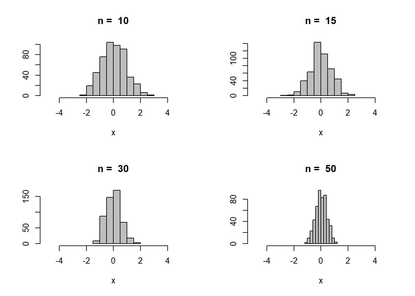
Generally you should observe that for the smaller sample sizes the histogram looks roughly triangle shapes, but as the sample size increases it gets “skinnier” and looks more bell shaped.