Chapter 11 Statistical Analysis in R
Now we are going to cover how to perform a variety of basic statistical tests in R.
- Proportion tests
- Chi-squared
- Fisher’s Exact Test
- Correlation
- T-tests/Rank-sum tests
- One-way ANOVA/Kruskal-Wallis
- Linear Regression
- Logistic Regression
- Poisson Regression
Note: We will be glossing over the statistical theory and “formulas” for these tests. There are plenty of resources online for learning more about these tests if you have not had a course covering this material. You will only be required to write code to fit or perform these test but will not be expected to interpret the results for this course.
11.1 Proportion tests
prop.test() can be used for testing the null that the proportions (probabilities of success) in several groups are the same, or that they equal certain given values.
prop.test(x, n, p = NULL,
          alternative = c("two.sided", "less", "greater"),
          conf.level = 0.95, correct = TRUE)
    1-sample proportions test with continuity correction

data:  15 out of 32, null probability 0.5
X-squared = 0.03125, df = 1, p-value = 0.8597
alternative hypothesis: true p is not equal to 0.5
95 percent confidence interval:
 0.2951014 0.6496695
sample estimates:
      p
0.46875
11.2 Chi-squared tests
chisq.test() performs chi-squared contingency table tests and goodness-of-fit tests.
chisq.test(x, y = NULL, correct = TRUE,
           p = rep(1/length(x), length(x)), rescale.p = FALSE,
           simulate.p.value = FALSE, B = 2000)
Let’s look at example using the cars data.
library(readr)
cars = read_csv("data/kaggleCarAuction.csv",
  col_types = cols(VehBCost = col_double()))
head(cars)
# A tibble: 6 × 34
RefId IsBadBuy PurchDate Auction VehYear VehicleAge Make Model Trim SubModel
<dbl> <dbl> <chr> <chr> <dbl> <dbl> <chr> <chr> <chr> <chr>
1 1 0 12/7/2009 ADESA 2006 3 MAZDA MAZD… i 4D SEDA…
2 2 0 12/7/2009 ADESA 2004 5 DODGE 1500… ST QUAD CA…
3 3 0 12/7/2009 ADESA 2005 4 DODGE STRA… SXT 4D SEDA…
4 4 0 12/7/2009 ADESA 2004 5 DODGE NEON SXT 4D SEDAN
5 5 0 12/7/2009 ADESA 2005 4 FORD FOCUS ZX3 2D COUP…
6 6 0 12/7/2009 ADESA 2004 5 MITS… GALA… ES 4D SEDA…
# ℹ 24 more variables: Color <chr>, Transmission <chr>, WheelTypeID <chr>,
# WheelType <chr>, VehOdo <dbl>, Nationality <chr>, Size <chr>,
# TopThreeAmericanName <chr>, MMRAcquisitionAuctionAveragePrice <chr>,
# MMRAcquisitionAuctionCleanPrice <chr>,
# MMRAcquisitionRetailAveragePrice <chr>,
# MMRAcquisitonRetailCleanPrice <chr>, MMRCurrentAuctionAveragePrice <chr>,
# MMRCurrentAuctionCleanPrice <chr>, MMRCurrentRetailAveragePrice <chr>, …
        0     1
  0 62375  1632
  1  8763   213
You can also pass in a table object (such as tab here)
    Pearson's Chi-squared test with Yates' continuity correction

data:  tab
X-squared = 0.92735, df = 1, p-value = 0.3356[1] "statistic" "parameter" "p.value" "method" "data.name" "observed"
[7] "expected" "residuals" "stdres" [1] 0.3355516Note that does the same test as prop.test, for a 2x2 table (prop.test not relevant for greater than 2x2).
    Pearson's Chi-squared test with Yates' continuity correction

data:  tab
X-squared = 0.92735, df = 1, p-value = 0.3356
    2-sample test for equality of proportions with continuity correction

data:  tab
X-squared = 0.92735, df = 1, p-value = 0.3356
alternative hypothesis: two.sided
95 percent confidence interval:
 -0.005208049  0.001673519
sample estimates:
   prop 1    prop 2
0.9745028 0.9762701
11.3 Fisher’s Exact test
fisher.test() performs contingency table test using the hypergeometric distribution (used for small sample sizes).
fisher.test(x, y = NULL, workspace = 200000, hybrid = FALSE,
            control = list(), or = 1, alternative = "two.sided",
            conf.int = TRUE, conf.level = 0.95,
            simulate.p.value = FALSE, B = 2000)
    Fisher's Exact Test for Count Data

data:  tab
p-value = 0.3324
alternative hypothesis: true odds ratio is not equal to 1
95 percent confidence interval:
 0.8001727 1.0742114
sample estimates:
odds ratio
 0.9289923
11.4 Correlation
cor() performs correlation in R
cor(x, y = NULL, use = "everything",
    method = c("pearson", "kendall", "spearman"))
Like other functions, if there are NAs, you get NA as the result. But if you specify use only the complete observations, then it will give you correlation on the non-missing data.
library(readr)
circ = read_csv("./data/Charm_City_Circulator_Ridership.csv")
cor(circ$orangeAverage, circ$purpleAverage, use="complete.obs")
[1] 0.9195356You can also get the correlation between matrix columns
select: dropped 11 variables (day, date, orangeBoardings, orangeAlightings, purpleBoardings, …) orangeAverage purpleAverage greenAverage bannerAverage
orangeAverage 1.000 0.908 0.840 0.545
purpleAverage 0.908 1.000 0.867 0.521
greenAverage 0.840 0.867 1.000 0.453
bannerAverage 0.545 0.521 0.453 1.000Or between columns of two matrices/dfs, column by column.
select: dropped 2 variables (greenAverage, bannerAverage)select: dropped 2 variables (orangeAverage, purpleAverage) greenAverage bannerAverage
orangeAverage 0.840 0.545
purpleAverage 0.867 0.521You can also use cor.test() to test for whether correlation is significant (ie non-zero). Note that linear regression may be better, especially if you want to regress out other confounders.
    Pearson's product-moment correlation

data:  circ$orangeAverage and circ$purpleAverage
t = 73.656, df = 991, p-value < 2.2e-16
alternative hypothesis: true correlation is not equal to 0
95 percent confidence interval:
 0.9093438 0.9286245
sample estimates:
      cor
0.9195356
For many of these testing result objects, you can extract specific slots/results as numbers, as the ct object is just a list.
List of 9
 $ statistic  : Named num 73.7
  ..- attr(*, "names")= chr "t"
 $ parameter  : Named int 991
  ..- attr(*, "names")= chr "df"
 $ p.value    : num 0
 $ estimate   : Named num 0.92
  ..- attr(*, "names")= chr "cor"
 $ null.value : Named num 0
  ..- attr(*, "names")= chr "correlation"
 $ alternative: chr "two.sided"
 $ method     : chr "Pearson's product-moment correlation"
 $ data.name  : chr "circ$orangeAverage and circ$purpleAverage"
 $ conf.int   : num [1:2] 0.909 0.929
  ..- attr(*, "conf.level")= num 0.95
- attr(*, "class")= chr "htest"[1] "statistic" "parameter" "p.value" "estimate" "null.value"
[6] "alternative" "method" "data.name" "conf.int" t
73.65553 [1] 0The broom package has a tidy function that puts most objects into data.frames so that they are easily manipulated:
# A tibble: 1 × 8
  estimate statistic p.value parameter conf.low conf.high method     alternative
     <dbl>     <dbl>   <dbl>     <int>    <dbl>     <dbl> <chr>      <chr>
1    0.920      73.7       0       991    0.909     0.929 Pearson's… two.sided
Note that you can add the correlation to a plot, via annotate
library(ggplot2)
txt = paste0("r=", signif(ct$estimate,3))
q = qplot(data = circ, x = orangeAverage, y = purpleAverage)
q + annotate("text", x = 4000, y = 8000, label = txt, size = 5)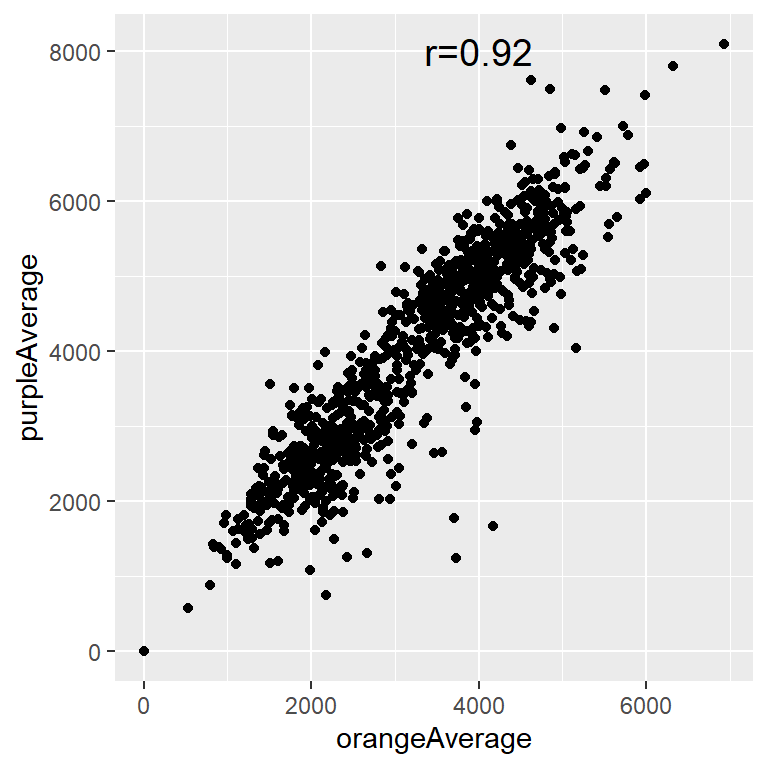
11.5 T-tests
The T-test is performed using the t.test() function, which essentially tests for the difference in means of a variable between two groups. It can perform a one sample t-test, two sample t-test, and a paired t-test.
In this syntax t.text(x, y)t, x and y are the columns of data for each group. It performs a two sample t-test assuming unequal variances.
    Welch Two Sample t-test

data:  circ$orangeAverage and circ$purpleAverage
t = -17.076, df = 1984, p-value < 2.2e-16
alternative hypothesis: true difference in means is not equal to 0
95 percent confidence interval:
 -1096.7602  -870.7867
sample estimates:
mean of x mean of y
 3033.161  4016.935
t.test saves a lot of information: the difference in means estimate, confidence interval for the difference conf.int, the p-value p.value, etc.
 [1] "statistic"   "parameter"   "p.value"     "conf.int"    "estimate"
 [6] "null.value"  "stderr"      "alternative" "method"      "data.name"
We can tidy this object into a data.frame with the tidy function.
# A tibble: 1 × 10
  estimate estimate1 estimate2 statistic  p.value parameter conf.low conf.high
     <dbl>     <dbl>     <dbl>     <dbl>    <dbl>     <dbl>    <dbl>     <dbl>
1    -984.     3033.     4017.     -17.1 4.20e-61     1984.   -1097.     -871.
# ℹ 2 more variables: method <chr>, alternative <chr>
You can also use the ‘formula’ notation. In this syntax, it is y ~ x, where x is a factor with 2 levels or a binary variable and y is a vector of the same length.
library(tidyr)
long = circ %>%
  select(date, orangeAverage, purpleAverage) %>%
  pivot_longer(-date, names_to = "line", values_to = "avg")
select: dropped 12 variables (day, orangeBoardings, orangeAlightings, purpleBoardings, purpleAlightings, …)pivot_longer: reorganized (orangeAverage, purpleAverage) into (line, avg) [was 1146x3, now 2292x3]# A tibble: 1 × 10
estimate estimate1 estimate2 statistic p.value parameter conf.low conf.high
<dbl> <dbl> <dbl> <dbl> <dbl> <dbl> <dbl> <dbl>
1 -984. 3033. 4017. -17.1 4.20e-61 1984. -1097. -871.
# ℹ 2 more variables: method <chr>, alternative <chr>To perform a two-sample t-test assuming equal variances, set var.equal = TRUE.
# A tibble: 1 × 10
  estimate estimate1 estimate2 statistic  p.value parameter conf.low conf.high
     <dbl>     <dbl>     <dbl>     <dbl>    <dbl>     <dbl>    <dbl>     <dbl>
1    -984.     3033.     4017.     -17.2 2.16e-62      2127   -1096.     -872.
# ℹ 2 more variables: method <chr>, alternative <chr>
This data is actually matched by date, so we should perform a paired t-test by setting paired = TRUE.
# A tibble: 1 × 8
  estimate statistic   p.value parameter conf.low conf.high method   alternative
     <dbl>     <dbl>     <dbl>     <dbl>    <dbl>     <dbl> <chr>    <chr>
1    -764.     -42.1 7.88e-223       992    -800.     -729. Paired … two.sided
11.6 Wilcoxon Rank-Sum Tests
Nonparametric analogue to the two sample t-test (testing medians or means if symmetric distributions):
# A tibble: 1 × 4
  statistic  p.value method                                          alternative
      <dbl>    <dbl> <chr>                                           <chr>
1   336714. 4.56e-58 Wilcoxon rank sum test with continuity correct… two.sided
11.7 Wilcoxon Signed Rank Test
Nonparametric analogue to the paired t-test (testing medians or means if symmetric distributions):
# A tibble: 1 × 4
  statistic   p.value method                                         alternative
      <dbl>     <dbl> <chr>                                          <chr>
1    17310. 2.16e-141 Wilcoxon signed rank test with continuity cor… two.sided
11.8 One-way ANOVA
You can fit an ANOVA model using the aov() function, using the formula notation y~x, where
yis your outcomexis your predictor
library(tidyr)
long2 = circ %>%
  select(date, orangeAverage, purpleAverage, greenAverage) %>%
  pivot_longer(-date, names_to = "line", values_to = "avg")
select: dropped 11 variables (day, orangeBoardings, orangeAlightings, purpleBoardings, purpleAlightings, …)pivot_longer: reorganized (orangeAverage, purpleAverage, greenAverage) into (line, avg) [was 1146x4, now 3438x3] Df Sum Sq Mean Sq F value Pr(>F)
line 2 1.443e+09 721298432 490 <2e-16 ***
Residuals 2611 3.843e+09 1471992
---
Signif. codes: 0 '***' 0.001 '**' 0.01 '*' 0.05 '.' 0.1 ' ' 1
824 observations deleted due to missingness11.9 Kruskal Wallis Test
Nonparametric analog to one-way ANOVA (testing medians or means if symmetric distributions):
    Kruskal-Wallis rank sum test

data:  avg by factor(line)
Kruskal-Wallis chi-squared = 729.07, df = 2, p-value < 2.2e-16
11.10 Linear Regression
Now we will briefly cover linear regression. I will use a little notation here so some of the commands are easier to put in the proper context. \[ y_i = \beta_0 + \beta x_i + \varepsilon_i \] where:
- \(y_i\) is the outcome for person i
- \(\beta_0\) is the intercept
- \(\beta_1\) is the slope
- \(x_i\) is the predictor for person i
- \(\varepsilon_i\) is the residual variation for person i
The R version of the regression model is:
y ~ x
where:
- y is your outcome
- x is/are your predictor(s)
For a linear regression, when the predictor is binary this is the same as a t-test:
Call:
lm(formula = avg ~ line, data = long)

Coefficients:
      (Intercept)  linepurpleAverage
3033.2 983.8 - ‘(Intercept)’ is \(\beta_0\)
- ‘linepurpleAverage’ is \(\beta_1\)
The summary command gets all the additional information (p-values, t-statistics, r-square) that you usually want from a regression.
Call:
lm(formula = avg ~ line, data = long)

Residuals:
    Min      1Q  Median      3Q     Max
-4016.9 -1121.2    64.3  1060.8  4072.6

Coefficients:
                  Estimate Std. Error t value Pr(>|t|)
(Intercept)        3033.16      38.99   77.79   <2e-16 ***
linepurpleAverage   983.77      57.09   17.23   <2e-16 ***
---
Signif. codes:  0 '***' 0.001 '**' 0.01 '*' 0.05 '.' 0.1 ' ' 1

Residual standard error: 1314 on 2127 degrees of freedom
  (163 observations deleted due to missingness)
Multiple R-squared:  0.1225,    Adjusted R-squared:  0.1221
F-statistic: 296.9 on 1 and 2127 DF,  p-value: < 2.2e-16
The coefficients from a summary are the coefficients, standard errors, t-statistics, and p-values for all the estimates.
 [1] "call"          "terms"         "residuals"     "coefficients"
 [5] "aliased"       "sigma"         "df"            "r.squared"
[9] "adj.r.squared" "fstatistic" "cov.unscaled" "na.action" Estimate Std. Error t value Pr(>|t|)
(Intercept) 3033.1611 38.98983 77.79365 0.000000e+00
linepurpleAverage 983.7735 57.09059 17.23180 2.163655e-62We can tidy linear models as well and it gives us all of this in one::
# A tibble: 2 × 5
  term              estimate std.error statistic  p.value
  <chr>                <dbl>     <dbl>     <dbl>    <dbl>
1 (Intercept)          3033.      39.0      77.8 0
2 linepurpleAverage     984.      57.1      17.2 2.16e-62
Let’s look at an example using the Kaggle car auction data. We’ll look at vehicle odometer value by vehicle age:
Call:
lm(formula = VehOdo ~ VehicleAge, data = cars)

Coefficients:
(Intercept)   VehicleAge
      60127         2723
Note that you can have more than 1 predictor in regression models. The interpretation for each slope is average change in the outcome corresponding to a one-unit change in the predictor, holding all other predictors constant.
Call:
lm(formula = VehOdo ~ IsBadBuy + VehicleAge, data = cars)

Residuals:
   Min     1Q Median     3Q    Max
-70856  -9490   1390  10311  41193

Coefficients:
            Estimate Std. Error t value Pr(>|t|)
(Intercept) 60141.77     134.75  446.33   <2e-16 ***
IsBadBuy     1329.00     157.84    8.42   <2e-16 ***
VehicleAge   2680.33      30.27   88.53   <2e-16 ***
---
Signif. codes:  0 '***' 0.001 '**' 0.01 '*' 0.05 '.' 0.1 ' ' 1

Residual standard error: 13810 on 72980 degrees of freedom
Multiple R-squared:  0.1031,    Adjusted R-squared:  0.1031
F-statistic:  4196 on 2 and 72980 DF,  p-value: < 2.2e-16
The * does interactions:
Call:
lm(formula = VehOdo ~ IsBadBuy * VehicleAge, data = cars)

Residuals:
   Min     1Q Median     3Q    Max
-70857  -9490   1391  10311  41193

Coefficients:
                    Estimate Std. Error t value Pr(>|t|)
(Intercept)         60139.70     143.23 419.872  < 2e-16 ***
IsBadBuy             1347.28     456.23   2.953  0.00315 **
VehicleAge           2680.84      32.54  82.380  < 2e-16 ***
IsBadBuy:VehicleAge    -3.79      88.74  -0.043  0.96594
---
Signif. codes:  0 '***' 0.001 '**' 0.01 '*' 0.05 '.' 0.1 ' ' 1

Residual standard error: 13810 on 72979 degrees of freedom
Multiple R-squared:  0.1031,    Adjusted R-squared:  0.1031
F-statistic:  2798 on 3 and 72979 DF,  p-value: < 2.2e-16
You can take out main effects with minus
Call:
lm(formula = VehOdo ~ IsBadBuy * VehicleAge - IsBadBuy, data = cars)

Residuals:
   Min     1Q Median     3Q    Max
-70822  -9493   1389  10311  41172

Coefficients:
                    Estimate Std. Error t value Pr(>|t|)
(Intercept)         60272.49     136.00 443.184  < 2e-16 ***
VehicleAge           2652.94      31.14  85.186  < 2e-16 ***
IsBadBuy:VehicleAge   242.08      30.70   7.885 3.19e-15 ***
---
Signif. codes:  0 '***' 0.001 '**' 0.01 '*' 0.05 '.' 0.1 ' ' 1

Residual standard error: 13810 on 72980 degrees of freedom
Multiple R-squared:  0.103, Adjusted R-squared:  0.103
F-statistic:  4192 on 2 and 72980 DF,  p-value: < 2.2e-16
Factors get special treatment in regression models - lowest level of the factor is the comparison group, and all other factors are relative to its values.
Call:
lm(formula = VehOdo ~ factor(TopThreeAmericanName), data = cars)

Residuals:
   Min     1Q Median     3Q    Max
-71947  -9634   1532  10472  45936

Coefficients:
                                  Estimate Std. Error t value Pr(>|t|)
(Intercept)                       68248.48      92.98 733.984  < 2e-16 ***
factor(TopThreeAmericanName)FORD   8523.49     158.35  53.828  < 2e-16 ***
factor(TopThreeAmericanName)GM     4952.18     128.99  38.393  < 2e-16 ***
factor(TopThreeAmericanName)NULL  -2004.68    6361.60  -0.315 0.752670
factor(TopThreeAmericanName)OTHER   584.87     159.92   3.657 0.000255 ***
---
Signif. codes:  0 '***' 0.001 '**' 0.01 '*' 0.05 '.' 0.1 ' ' 1

Residual standard error: 14220 on 72978 degrees of freedom
Multiple R-squared:  0.04822,   Adjusted R-squared:  0.04817
F-statistic: 924.3 on 4 and 72978 DF,  p-value: < 2.2e-16
Some additional generic functions that are useful when working with linear regression models are
residuals- extract the residuals from a model fitpredict- make predictions based on a model fit. Can make predictions for data used to fit the model (returning the fitted values) or for a new observation.
We can extract the residuals for calculations or residual plots for diagnostics. For example, let’s make a histogram of the residuals from the cars model fit3.
fit3.res = data.frame(resid = residuals(fit3))
library(ggplot2)
ggplot(fit3.res, aes(x = resid)) + geom_histogram()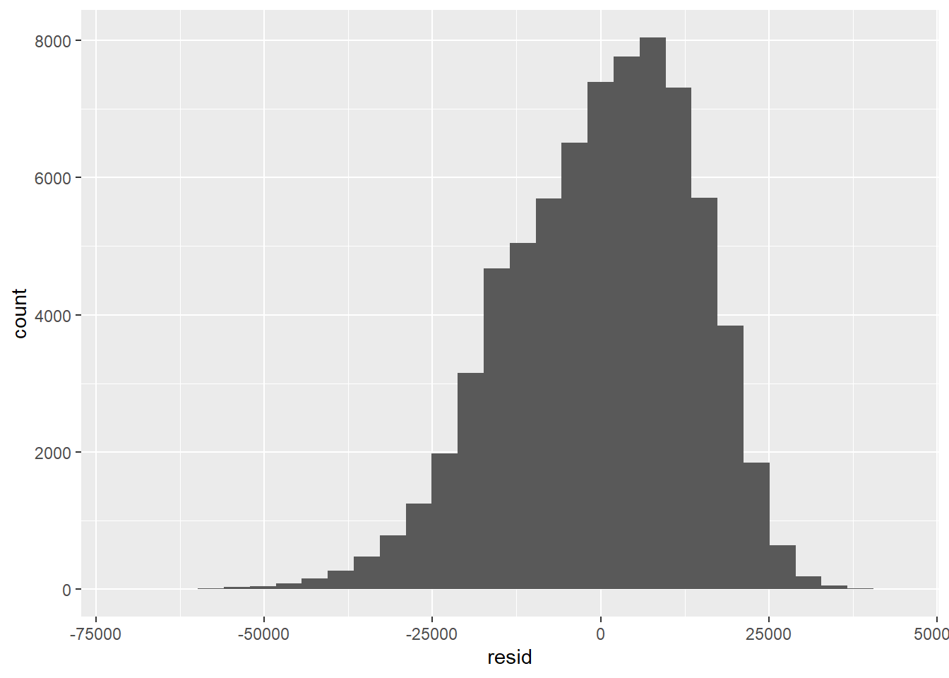
We can also predict the mean odometer reading for a car that is a bad buy and is 4 years old using the model fit3, we create a data.frame containing these two columns with the values 1 (is a bad buy) and 4 to use with predict.
new_data = data.frame(IsBadBuy = 1, VehicleAge = 4)
predict(fit3, newdata = new_data, interval = "confidence")
fit lwr upr
1 72195.17 71871.49 72518.85 fit lwr upr
1 72195.17 45131.74 99258.611.11 Logistic Regression and GLMs
Generalized Linear Models (GLMs) allow for fitting regressions for non-continuous/normal outcomes. The glm has similar syntax to the lm command. Logistic regression is one example.
In a (simple) logistic regression model, we have a binary response Y and a predictor x. It is assumed that given the predictor, \(Y\sim \text{Bernoulli}(p(x))\) where \(p(x) = P(Y=1|x)\) and
\[\log\left(\frac{P(Y=1|x)}{1-P(Y=1|x)}\right)=\beta_0+\beta_1x.\]
That is the log-odds of success changes linearly with x. It then follows that \(e^{\beta_1}\) is the odds ratio of success for a one unit increase in x.
Call:
glm(formula = IsBadBuy ~ VehOdo + VehicleAge, family = binomial(),
    data = cars)

Coefficients:
              Estimate Std. Error z value Pr(>|z|)
(Intercept) -3.778e+00  6.381e-02 -59.211   <2e-16 ***
VehOdo       8.341e-06  8.526e-07   9.783   <2e-16 ***
VehicleAge   2.681e-01  6.772e-03  39.589   <2e-16 ***
---
Signif. codes:  0 '***' 0.001 '**' 0.01 '*' 0.05 '.' 0.1 ' ' 1

(Dispersion parameter for binomial family taken to be 1)

    Null deviance: 54421  on 72982  degrees of freedom
Residual deviance: 52346  on 72980  degrees of freedom
AIC: 52352

Number of Fisher Scoring iterations: 5
We can tidy this model fit object as well. Use conf.int = TRUE to get confidence intervals for the regression coefficients.
# A tibble: 3 × 7
  term           estimate   std.error statistic  p.value    conf.low  conf.high
  <chr>             <dbl>       <dbl>     <dbl>    <dbl>       <dbl>      <dbl>
1 (Intercept) -3.78       0.0638         -59.2  0        -3.90       -3.65
2 VehOdo       0.00000834 0.000000853      9.78 1.33e-22  0.00000667  0.0000100
3 VehicleAge   0.268      0.00677         39.6  0         0.255       0.281
Use the conf.int = TRUE and exponentiate = TRUE to get the confidence intervals and point estimates for the odds ratios.
# A tibble: 3 × 7
  term        estimate   std.error statistic  p.value conf.low conf.high
  <chr>          <dbl>       <dbl>     <dbl>    <dbl>    <dbl>     <dbl>
1 (Intercept)   0.0229 0.0638         -59.2  0          0.0202    0.0259
2 VehOdo        1.00   0.000000853      9.78 1.33e-22   1.00      1.00
3 VehicleAge    1.31   0.00677         39.6  0          1.29      1.32
Note the coefficients are on the original scale, we must exponentiate them for odds ratios:
(Intercept)      VehOdo  VehicleAge
 0.02286316  1.00000834  1.30748911
11.12 Poisson Regression
Poisson regression is used for count responses. This model assumes that (in the case of a single predictor) that \(Y|x\sim \text{Poisson}(\lambda(x))\), where \(\lambda(x)=E[Y|x]\), and
\[\log(E[Y|x]) = \beta_0+\beta_1x.\]
Then \(e^{\beta_1}\) represents the rate ratio for a one unit increase in x. Note: An offset can be included in the formula by using offset(log(x))
Call:
glm(formula = orangeBoardings ~ day, family = poisson(), data = circ)

Coefficients:
              Estimate Std. Error z value Pr(>|z|)
(Intercept)   8.227920   0.001308 6288.15   <2e-16 ***
dayMonday    -0.196414   0.001948 -100.81   <2e-16 ***
daySaturday  -0.269110   0.001999 -134.61   <2e-16 ***
daySunday    -0.689711   0.002289 -301.37   <2e-16 ***
dayThursday  -0.152273   0.001932  -78.83   <2e-16 ***
dayTuesday   -0.171878   0.001939  -88.66   <2e-16 ***
dayWednesday -0.139633   0.001925  -72.53   <2e-16 ***
---
Signif. codes:  0 '***' 0.001 '**' 0.01 '*' 0.05 '.' 0.1 ' ' 1

(Dispersion parameter for poisson family taken to be 1)

    Null deviance: 573304  on 1078  degrees of freedom
Residual deviance: 465777  on 1072  degrees of freedom
  (67 observations deleted due to missingness)
AIC: 476293

Number of Fisher Scoring iterations: 4
11.13 Exercises
These exercises will use the child mortality dataset, indicatordeadkids35.csv, and the Kaggle car auction dataset, kaggleCarAuction.csv. Modify the following code to read in this dataset.
mort = read_csv("./data/indicatordeadkids35.csv")
mort = mort %>%
  rename(country = X1)
cars = read_csv("./data/kaggleCarAuction.csv",
col_types = cols(VehBCost = col_double()))- Compute the correlation between the
1980,1990,2000, and2010mortality data. No need to save this in an object. Just display the result to the screen. Note anyNAs. Then compute usinguse = "complete.obs". - Compute the correlation between the
Myanmar,China, andUnited Statesmortality data. Store this correlation matrix in an object calledcountry_cor - Extract the Myanmar-US correlation from the correlation matrix.
- Compute the correlation between the
- Is there a difference between mortality information from
1990and2000? Run a paired t-test and a Wilcoxon signed rank test to assess this. Hint: to extract the column of information for1990, usemort$"1990" - Using the cars dataset, fit a linear regression model with vehicle cost (
VehBCost) as the outcome and vehicle age (VehicleAge) and whether it’s an online sale (IsOnlineSale) as predictors as well as their interaction. Save the model fit in an object calledlmfit_carsand display the summary table. - Create a variable called
expensivein thecarsdata that indicates if the vehicle cost is over$10,000. Use a chi-squared test to assess if there is a relationship between a car being expensive and it being labeled as a “bad buy” (IsBadBuy). - Fit a logistic regression model where the outcome is “bad buy” status and predictors are the
expensivestatus and vehicle age (VehicleAge). Save the model fit in an object calledlogfit_carsand display the summary table. Use summary ortidy(logfit_cars, conf.int = TRUE, exponentiate = TRUE)ortidy(logfit_cars, conf.int = TRUE, exponentiate = FALSE)for log odds ratios