Chapter 2 RStudio
RStudio is an IDE that provides features to make using and managing R much easier. Let’s take a look at base R first.
2.1 Base R
To work with base R, you have access to two ways to write and run your code:
- The R console - this is the “interpreter” and runs your code in real time (as opposed to needing to compile your code and then run it). It interprets whatever you write into the console to
- Perform basic calculations such as
2 + 2 - Assign values to a variable
- Apply a function
- Perform basic calculations such as
- R scripts - An R analysis script allows you to store your code in a static document that you can save. A script allows you to
- Save your code and to share with others (reproducibility)
- Try things out interactively and then add/modify to your code in the script
R revolves around functions. These functions are commands that take input, perform computations, and return results. For example, we will learn to use the lm() function which takes in a dataset and a linear regression model formula and returns the linear regression model fit. When you download R, it has a “base” set of functions/packages (base R).
We can extend R, by installing packages, using install.packages("name_of_package"), from CRAN to gain access to new functions in R by then loading the library by using library(name_of_package). These packages are written by R users/developers (like us). Because packages can be made by any R users, some are bad. To learn more about knowing which packages to trust, take a look at this article in how to trust an R package. RStudio (the company) makes a lot of great packages. Hadley Wickham, an employee and developer at RStudio) is an authority on all things R and writes many packages and references on using them. We will learn to use base R, since you will need to understand base R syntax when looking at many examples and answers to help questions on the internet, but we will also learn a more modern way to do things using the tidyverse.
2.2 RStudio IDE
RStudio is an integrated development environment (IDE) for R. It helps the user effectively use R by making things easier. It is not a drop down statistical tool (suc as stata, minitab, or excel), but there are some limited versions of R like this (see Rcmdr or Radiant).
RStudio makes working with R easier by including features such as syntax highlighting, code completion, and smart indentation. In RStudio, you can also easily manage multiple working directories and projects. RStudio also contains a workspace browser and data viewer, plot history which allows zooming and flexible image export, integrated R help and documentation, and searchable command history. When starting to work with RStudio, you may find the RStudio cheat sheet very helpful.
Lets take a quick tour of RStudio (Note all images here borrowed from https://ayeimanol-r.net/2013/04/21/289/). When you open RStudio, you will see four window panes. In the bottom left, you will see the R console
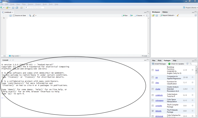 * This is where code is executed
* You can also type things here interactively
* Code is not saved on your disk when entered into the console
* This is where code is executed
* You can also type things here interactively
* Code is not saved on your disk when entered into the console
If you want to save your code, then use an R script. This will appear in top left corner of RStudio.
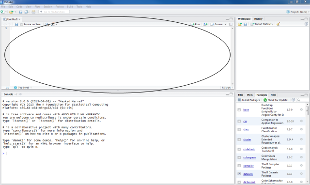 * R scripts (as well as other files such as Rmarkdown files) will open here
* You can add R code and comments to script files
* You can run the code from your script by highlighting the code and pressing CMD+Enter (Mac) or Ctrl+Enter (Windows).
* In .R files (R scripts), code is saved on your disk.
* R scripts (as well as other files such as Rmarkdown files) will open here
* You can add R code and comments to script files
* You can run the code from your script by highlighting the code and pressing CMD+Enter (Mac) or Ctrl+Enter (Windows).
* In .R files (R scripts), code is saved on your disk.
In the upper right hand side of RStudio is the workspace/environment pane.
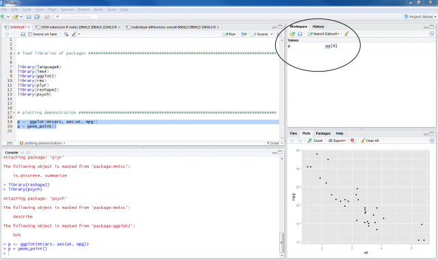
In this section, you can find
- Workspace/enviroment tab which tells you what objects are in R and what exists in memory/what is loaded/what you have read in.
- History tab which shows previous commands you have run. This is useful for debugging your code, but don’t rely on it as a script. (Note: you can also press the up arrow in the console to see previous code you have run.)
In the bottom right hand corner, there are several tabs which include
- Files - shows the files on your computer in the directory you are working in
- Viewer - can vew data or R objects
- Help - shows help documentations for R commands
- Plots - shows plots generated in your R sessions. Can see current and previous plots, save, and export them to png/pdf formats.
- Packages - list of R packages you have installed
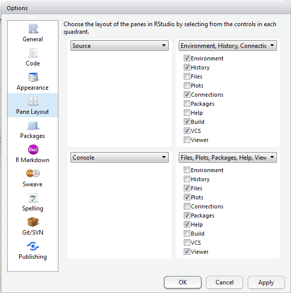
If you would like to rearrange these panes in RStudio (as I have), you can go to Tools > Global Options > Pane Layout and select the order you want the panes to appear.
 ## Some Useful Shortcuts in RStudio
- Ctrl+Enter (or CMD+Enter on Mac) will run the current line of code in an R script (the same as copying and pasting the code from your script to the R console).
- Ctlr+1 take you to the script page
- Ctrl+2 takes you to the consol
- See the RStudio keyboard shortcuts for additional shortcut commands.
2.3 R Projects and Intro to RMarkdown
R projects are a great way to manage all the files used in your R session. Creating an R project can be extremely helpful in orgranizing your work:
- Helps you organize your work.
- Helps with working directories (discussed later).
- Allows you to easily know which project you’re on.
- Allows a project folder to be zipped and sent to another R users who can unzip and pick up right where you left off.
To create a new Rproject go to File > New Project > New Directory > New Project.
RStudio also makes it easy to create RMarkdown documents, which are great for making reports. You can write a document that allows you to easily include both R code and output along with your documentation of the process.
Lets take a look at an example RMarkdown document. Download and unzip the RStudio lab folder from the CANVAS page and open the Rproject file in the unzipped folder. Below is what the rendered RMarkdown document will look like.
2.3.1 R Markdown
This is an R Markdown document. Markdown is a simple formatting syntax for authoring HTML, PDF, and MS Word documents. For more details on using R Markdown see http://rmarkdown.rstudio.com.
The way you can create a file like this in RStudio is: File → New File → R Markdown and then using the default or using a template.
When you click the Knit button a document will be generated that includes both content as well as the output of any embedded R code chunks within the document. You can embed an R code chunk like this:
2.3.2 Plotting some data
Here is code that will make a plot of the average daily ridership in Baltimore City for the Charm City Circulator: https://www.charmcitycirculator.com/.
Here we plot a few days:
# keep only some days
avg = avg %>%
  filter(day %in% c("Monday", "Tuesday", "Friday", "Saturday"))

palette = c(
  banner = "blue",
  green = "darkgreen",
  orange = "orange",
  purple = "purple")

ggplot(aes(x = date, y = number, colour = line), data= avg) +
  geom_line() +
  facet_wrap( ~day) +
  scale_colour_manual(values = palette)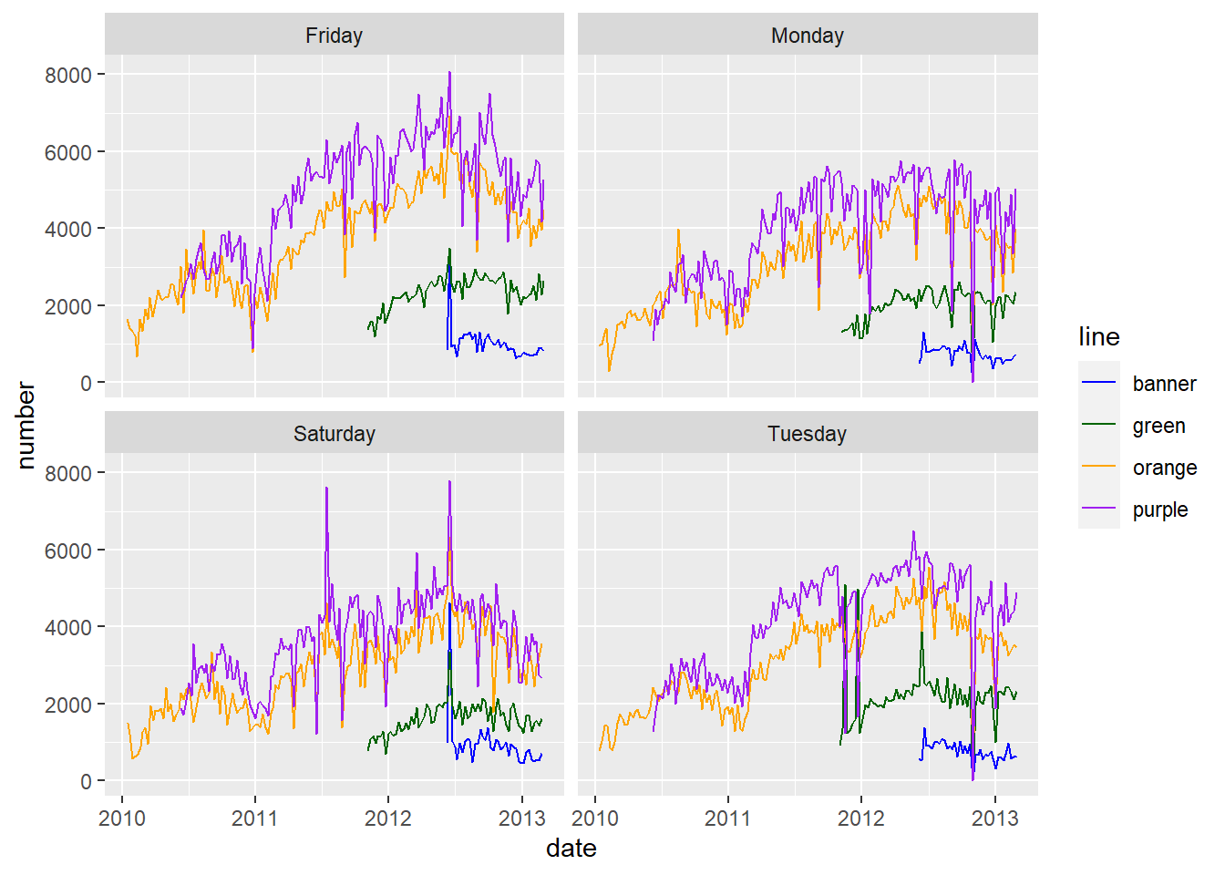
2.3.3 Exercise
Use the provided RProject with RMarkdown file (shown above) to begin exploring R. Here are a few changes that will show you how to change small things in R code and the output it makes. After each change, hit the Knit button again.
- Go through and change the colors in
paletteto something other than what they originally were. See http://www.stat.columbia.edu/~tzheng/files/Rcolor.pdf for a large list of colors. - Change the days you are keeping to show
"Sunday"instead of"Saturday". - Change the word
geom_line()togeom_point(). - Create another RMarkdown Document from RStudio dropdowns.