Chapter 14 RMarkdown

The three “back ticks” (`) must be followed by curly brackets “{”, and then “r” to tell the computer that you are using R code. This line is then closed off by another curly bracket “}”.

Anything before three more back ticks “```” are then considered R code (a script).

If any code in the document has just a backtick ` then nothing, then another backtick, then that word is just printed as if it were code, such as hey.

I’m reading in the bike lanes here.

# readin is just a "label" for this code chunk
## code chunk is just a "chunk" of code, where this code usually
## does just one thing, aka a module
### comments are still # here
### you can do all your reading in there
### let's say we loaded some packages
library(stringr)
library(dplyr)
library(tidyr)
library(readr)
fname <- "./data/Bike_Lanes.csv"
bike = read_csv(fname)

You can write your introduction here.

14.1 Introduction

Bike lanes are in Baltimore. People like them. Why are they so long?

14.2 Exploratory Analysis

Let’s look at some plots of bike length. Let’s say we wanted to look at what affects bike length.

14.2.1 Plots of bike length

Note we made the subsection by using three “hashes” (pound signs): ###.

We can turn off R code output by using echo = FALSE on the knitr code chunks.

filter: removed 126 rows (8%), 1,505 rows remaining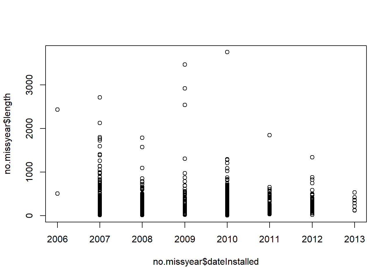

no.missyear = no.missyear %>%  mutate(dateInstalled = factor(dateInstalled)) 
library(ggplot2)
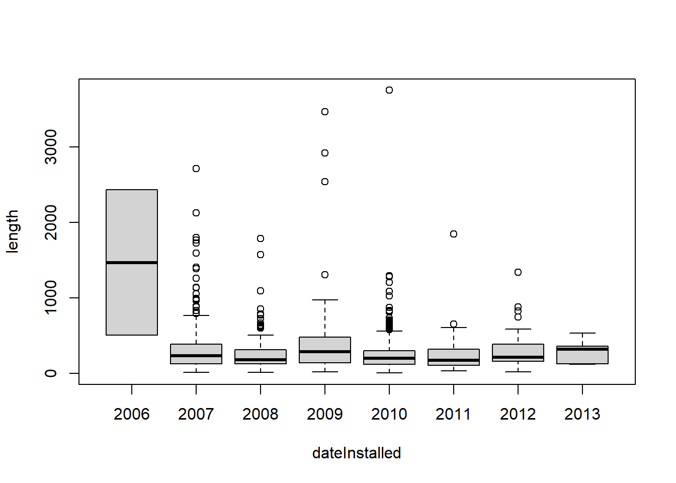
gbox = no.missyear %>% ggplot(aes(x = dateInstalled, y = length)) + geom_boxplot()
print(gbox)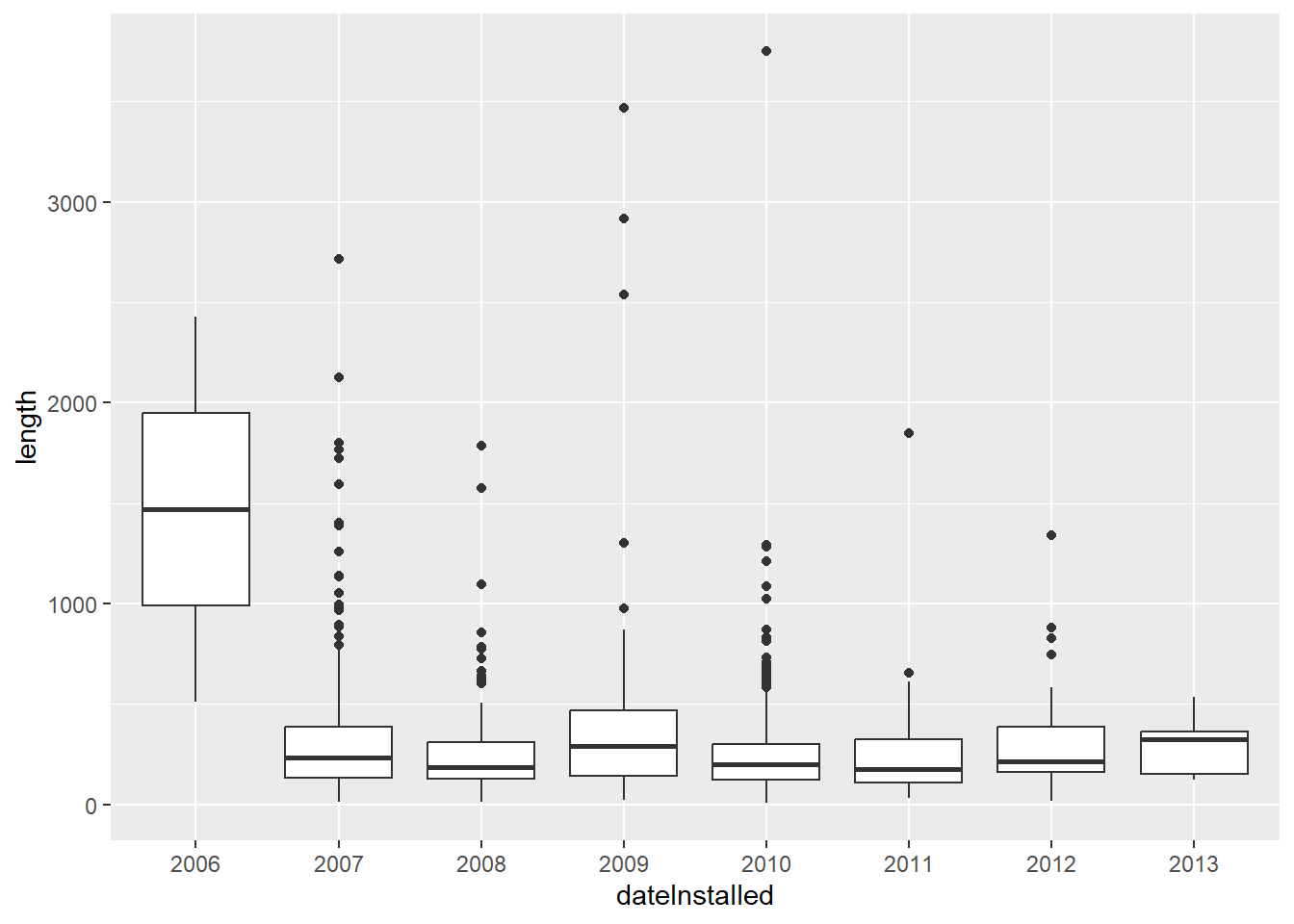

We have a total of 1505 rows.

What does it look like if we took the log (base 10) of the bike length:

no.missyear <- no.missyear %>% mutate(log.length = log10(length))
### see here that if you specify the data argument, you don't need to do the $ 
boxplot(log.length ~ dateInstalled, data = no.missyear, 
        main = "Boxplots of Bike Lenght by Year", 
        xlab="Year", 
        ylab="Bike Length")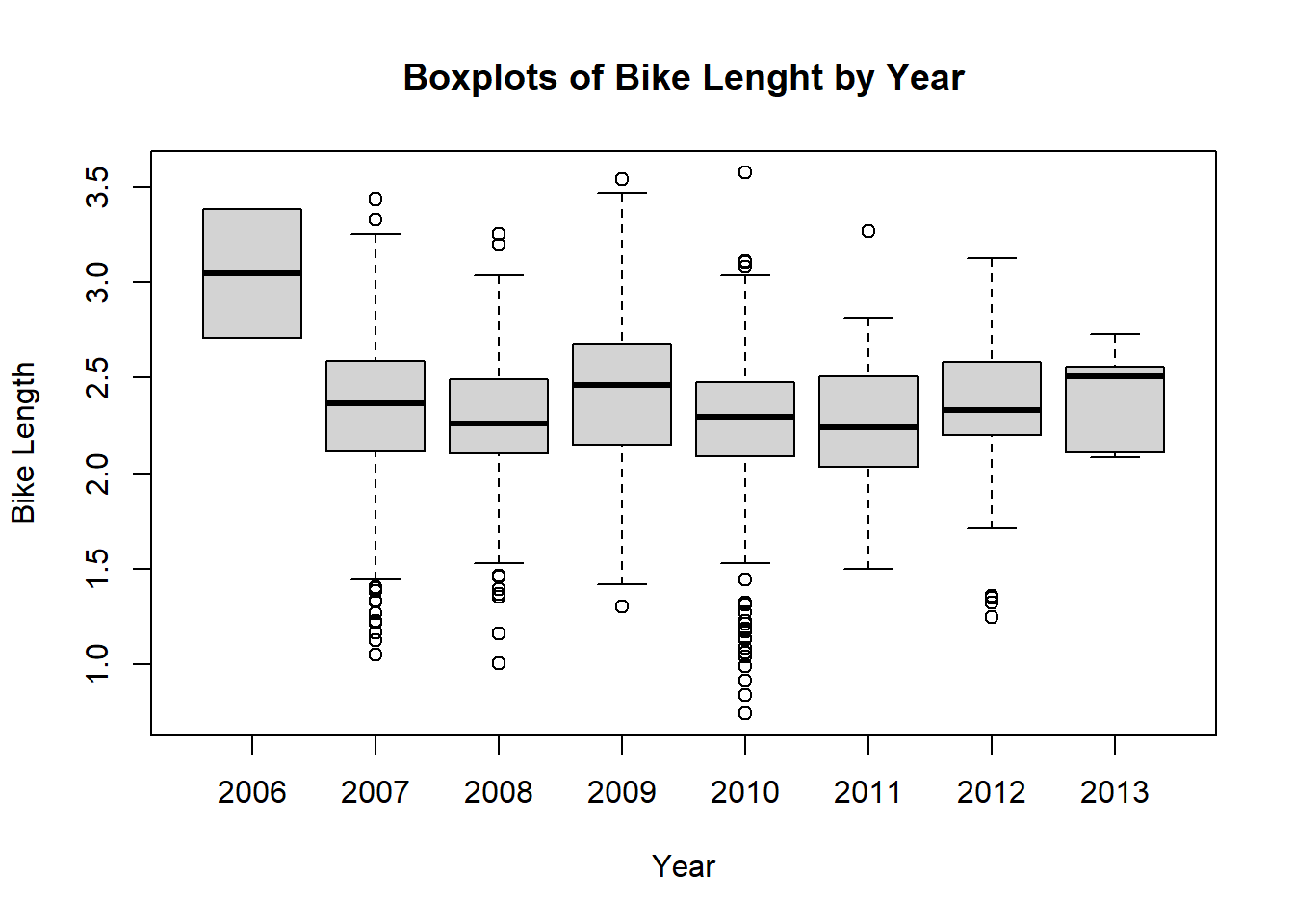

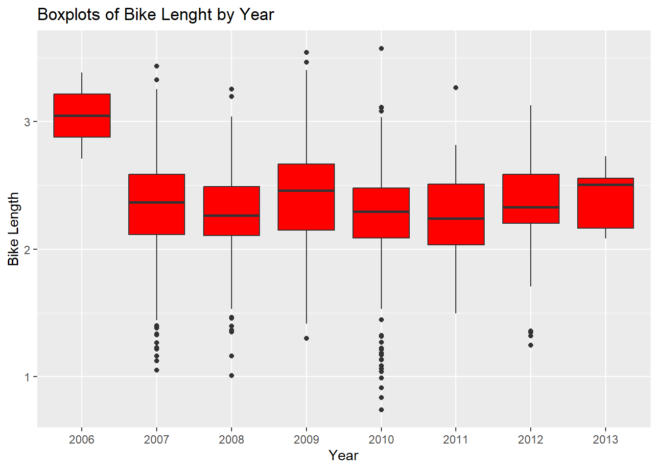
glogbox = no.missyear %>% ggplot(aes(x = dateInstalled, y = log.length)) + geom_boxplot() + 
  ggtitle("Boxplots of Bike Lenght by Year") + 
  xlab("Year") + 
  ylab("Bike Length")
print(glogbox)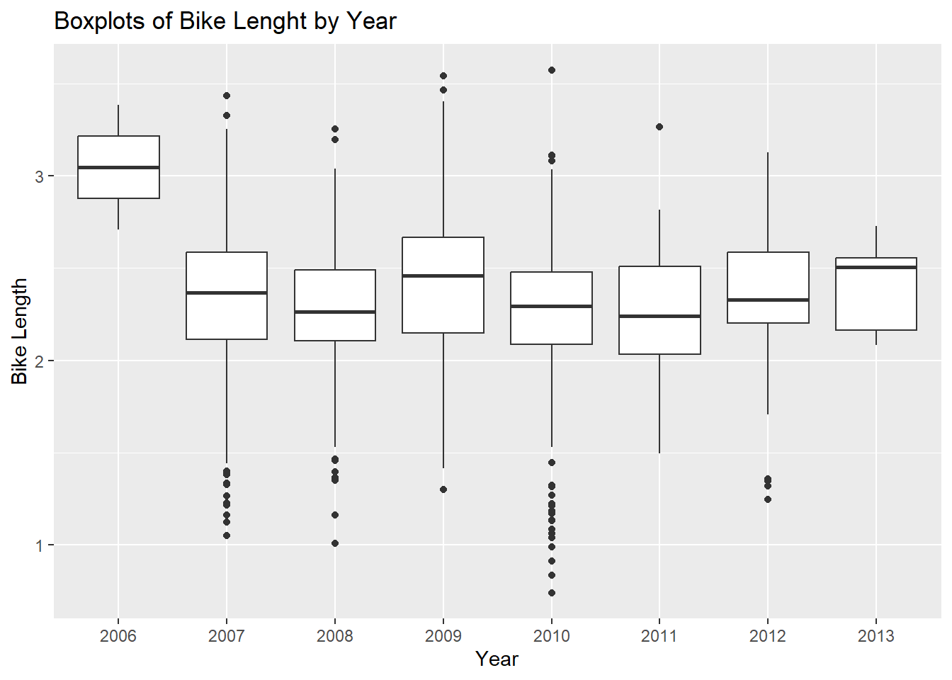

I want my boxplots colored, so I set the col argument.

boxplot(log.length ~ dateInstalled, 
        data=no.missyear, 
        main="Boxplots of Bike Lenght by Year",
        xlab="Year", 
        ylab="Bike Length", 
        col="red")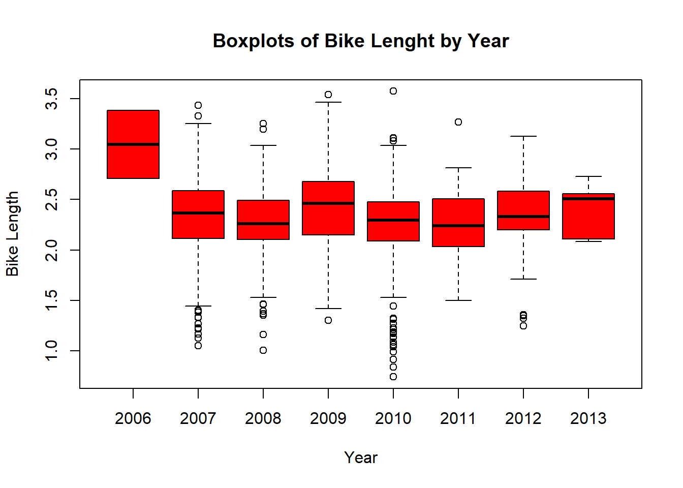

glogbox + geom_boxplot(fill = "red")

As we can see, 2006 had a much higher bike length. What about for the type of bike path?

### type is a character, but when R sees a "character" in a "formula", then it automatically converts it to factor
### a formula is something that has a y ~ x, which says I want to plot y against x
### or if it were a model you would do y ~ x, which meant regress against y
boxplot(log.length ~ type, data=no.missyear, main="Boxplots of Bike Lenght by Year", xlab="Year", ylab="Bike Length")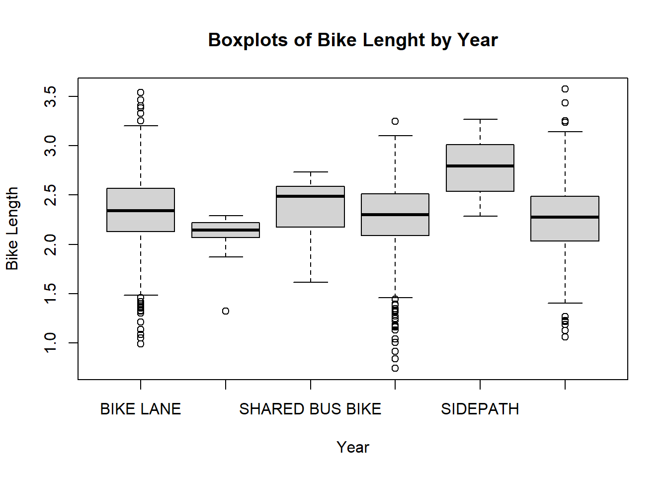

14.3 Multiple Facets

We can do the plot with different panels for each type.

glogbox + facet_wrap(~ type)

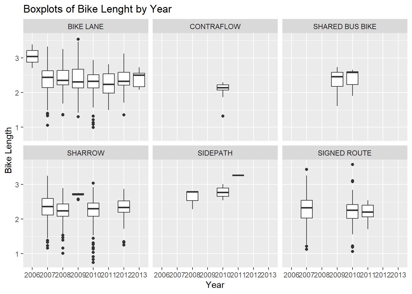
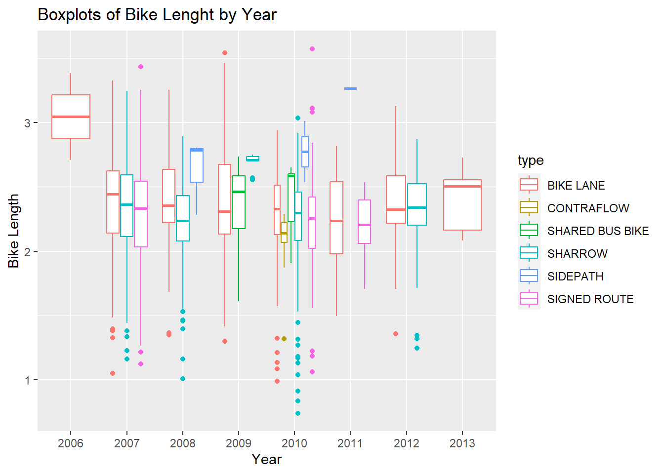
NOTE, this is different than if we colored on type:

glogbox + aes(colour = type)

14.3.1 Means by type

What if we want to extract means by each type?

Let’s show a few ways:

no.missyear %>% group_by(type) %>% 
  dplyr::summarise(mean = mean(log.length))

# A tibble: 6 × 2
  type             mean
  <chr>           <dbl>
1 BIKE LANE        2.33
2 CONTRAFLOW       2.09
3 SHARED BUS BIKE  2.36
4 SHARROW          2.26
5 SIDEPATH         2.78
6 SIGNED ROUTE     2.26

Let’s show a what if we wanted to go over type and dateInstalled:

no.missyear %>% group_by(type, dateInstalled) %>% 
  dplyr::summarise(mean = mean(log.length),
      median = median(log.length),
      Std.Dev = sd(log.length))

`summarise()` has grouped output by 'type'. You can override using
the `.groups` argument.

# A tibble: 22 × 5
# Groups:   type [6]
   type            dateInstalled  mean median Std.Dev
   <chr>           <fct>         <dbl>  <dbl>   <dbl>
 1 BIKE LANE       2006           3.05   3.05   0.480
 2 BIKE LANE       2007           2.35   2.44   0.407
 3 BIKE LANE       2008           2.37   2.35   0.389
 4 BIKE LANE       2009           2.38   2.31   0.494
 5 BIKE LANE       2010           2.31   2.33   0.321
 6 BIKE LANE       2011           2.24   2.24   0.334
 7 BIKE LANE       2012           2.36   2.32   0.285
 8 BIKE LANE       2013           2.41   2.51   0.240
 9 CONTRAFLOW      2010           2.09   2.14   0.257
10 SHARED BUS BIKE 2009           2.35   2.46   0.306
# ℹ 12 more rows

14.4 Linear Models

OK let’s do some linear model

### type is a character, but when R sees a "character" in a "formula", then it automatically converts it to factor
### a formula is something that has a y ~ x, which says I want to plot y against x
### or if it were a model you would do y ~ x, which meant regress against y
mod.type = lm(log.length ~ type, data = no.missyear)
mod.yr = lm(log.length ~ factor(dateInstalled), data = no.missyear)
mod.yrtype = lm(log.length ~ type + factor(dateInstalled), data = no.missyear)
summary(mod.type)


Call:
lm(formula = log.length ~ type, data = no.missyear)

Residuals:
     Min       1Q   Median       3Q      Max 
-1.51498 -0.19062  0.02915  0.23220  1.31021 

Coefficients:
                    Estimate Std. Error t value Pr(>|t|)    
(Intercept)          2.33061    0.01487 156.703  < 2e-16 ***
typeCONTRAFLOW      -0.24337    0.10288  -2.366 0.018127 *  
typeSHARED BUS BIKE  0.03239    0.06062   0.534 0.593194    
typeSHARROW         -0.07419    0.02129  -3.484 0.000509 ***
typeSIDEPATH         0.45122    0.15058   2.997 0.002775 ** 
typeSIGNED ROUTE    -0.06687    0.02726  -2.453 0.014300 *  
---
Signif. codes:  0 '***' 0.001 '**' 0.01 '*' 0.05 '.' 0.1 ' ' 1

Residual standard error: 0.367 on 1499 degrees of freedom
Multiple R-squared:  0.01956,   Adjusted R-squared:  0.01629 
F-statistic:  5.98 on 5 and 1499 DF,  p-value: 1.74e-05

That’s rather UGLY, so let’s use a package called pander and then make this model into an pander object and then print it out nicely.

14.5 Grabbing coefficients

We can use the coef function on a summary, or do smod$coef to get the coefficients. But they are in a matrix:

smod = summary(mod.type)
coef(smod)

                       Estimate Std. Error     t value     Pr(>|t|)
(Intercept)          2.33061129 0.01487281 156.7027729 0.0000000000
typeCONTRAFLOW      -0.24336564 0.10287662  -2.3656069 0.0181272020
typeSHARED BUS BIKE  0.03239334 0.06062453   0.5343274 0.5931943055
typeSHARROW         -0.07418617 0.02129463  -3.4837969 0.0005085795
typeSIDEPATH         0.45121749 0.15057577   2.9966142 0.0027748128
typeSIGNED ROUTE    -0.06686556 0.02726421  -2.4525034 0.0142999055

class(coef(smod))

[1] "matrix" "array"

14.5.1 Broom package

The broom package can “tidy” up the output to actually put the terms into a column of a data.frame that you can grab values from:

library(broom)
smod2 = tidy(mod.type)
class(smod2)

[1] "tbl_df"     "tbl"        "data.frame"

better = smod2 %>% mutate(term = str_replace(term, "^type", ""))
better

# A tibble: 6 × 5
  term            estimate std.error statistic  p.value
  <chr>              <dbl>     <dbl>     <dbl>    <dbl>
1 (Intercept)       2.33      0.0149   157.    0       
2 CONTRAFLOW       -0.243     0.103     -2.37  0.0181  
3 SHARED BUS BIKE   0.0324    0.0606     0.534 0.593   
4 SHARROW          -0.0742    0.0213    -3.48  0.000509
5 SIDEPATH          0.451     0.151      3.00  0.00277 
6 SIGNED ROUTE     -0.0669    0.0273    -2.45  0.0143

better %>% filter(term == "SIDEPATH")

filter: removed 5 rows (83%), one row remaining

# A tibble: 1 × 5
  term     estimate std.error statistic p.value
  <chr>       <dbl>     <dbl>     <dbl>   <dbl>
1 SIDEPATH    0.451     0.151      3.00 0.00277

write.csv(better, file = "Best_Model_Coefficients.csv")

BUT I NEEEEEED an XLSX! The xlsx package can do it, but I still tend to use CSVs. May need to look at this post if getting “Reason: image not found” error.

library(openxlsx) # may need to run sudo R CMD javareconf
write.xlsx(better, file = "Best_Model_Coefficients.xlsx")

14.5.2 Testing Nested Models

The anova command will test nested models and give you a table of results:

my_lrtest = anova(mod.yrtype, mod.yr)
print(my_lrtest)

Analysis of Variance Table

Model 1: log.length ~ type + factor(dateInstalled)
Model 2: log.length ~ factor(dateInstalled)
  Res.Df    RSS Df Sum of Sq     F   Pr(>F)    
1   1492 199.10                                
2   1497 202.47 -5   -3.3681 5.048 0.000136 ***
---
Signif. codes:  0 '***' 0.001 '**' 0.01 '*' 0.05 '.' 0.1 ' ' 1

print(tidy(my_lrtest))

# A tibble: 2 × 7
  term                          df.residual   rss    df sumsq statistic  p.value
  <chr>                               <dbl> <dbl> <dbl> <dbl>     <dbl>    <dbl>
1 log.length ~ type + factor(d…        1492  199.    NA NA        NA    NA      
2 log.length ~ factor(dateInst…        1497  202.    -5 -3.37      5.05  1.36e-4

Similarly with year:

my_lrtest = anova(mod.yrtype, mod.type)
print(tidy(my_lrtest))

# A tibble: 2 × 7
  term                          df.residual   rss    df sumsq statistic  p.value
  <chr>                               <dbl> <dbl> <dbl> <dbl>     <dbl>    <dbl>
1 log.length ~ type + factor(d…        1492  199.    NA NA        NA    NA      
2 log.length ~ type                    1499  202.    -7 -2.83      3.03  0.00359

ASIDE: the aov function fits what you think of when you think ANOVA.

14.6 Pander

Pander can output tables (as well as other things such as models), so let’s print this using the pander command from the pander package. So pander is really good when you are trying to print out a table (in html, otherwise make the table and use write.csv to get it in Excel and then format) really quickly and in a report.

# devtools::install_github('Rapporter/pander') # need this version!
library(pander)
pander(mod.yr)

Fitting linear model: log.length ~ factor(dateInstalled)
	Estimate	Std. Error	t value	Pr(>\|t\|)
(Intercept)	3.046	0.26	11.71	2.181e-30
factor(dateInstalled)2007	-0.7332	0.2608	-2.812	0.004987
factor(dateInstalled)2008	-0.7808	0.2613	-2.988	0.002852
factor(dateInstalled)2009	-0.6394	0.2631	-2.431	0.01518
factor(dateInstalled)2010	-0.7791	0.2605	-2.991	0.002825
factor(dateInstalled)2011	-0.8022	0.2626	-3.055	0.002292
factor(dateInstalled)2012	-0.7152	0.2625	-2.725	0.006509
factor(dateInstalled)2013	-0.638	0.2849	-2.239	0.02527

It is the same if we write out the summary, but more information is in the footer.

pander(summary(mod.yr))

	Estimate	Std. Error	t value	Pr(>\|t\|)
(Intercept)	3.046	0.26	11.71	2.181e-30
factor(dateInstalled)2007	-0.7332	0.2608	-2.812	0.004987
factor(dateInstalled)2008	-0.7808	0.2613	-2.988	0.002852
factor(dateInstalled)2009	-0.6394	0.2631	-2.431	0.01518
factor(dateInstalled)2010	-0.7791	0.2605	-2.991	0.002825
factor(dateInstalled)2011	-0.8022	0.2626	-3.055	0.002292
factor(dateInstalled)2012	-0.7152	0.2625	-2.725	0.006509
factor(dateInstalled)2013	-0.638	0.2849	-2.239	0.02527

Fitting linear model: log.length ~ factor(dateInstalled)
Observations	Residual Std. Error	$R^2$	Adjusted $R^2$
1505	0.3678	0.01697	0.01237

14.6.1 Formatting

Let’s format the rows and the column names a bit better:

14.6.1.1 Changing the terms

ptable = tidy(mod.yr)
ptable$term = ptable$term %>% 
  str_replace(fixed("factor(dateInstalled)"), "") %>%
  str_replace(fixed("(Intercept)"), "Intercept")

14.6.1.2 Column Names

Now we can reset the column names if we didn’t like them before:

colnames(ptable) = c("Variable", "Beta", "SE", "tstatistic", "p.value")
pander(ptable)

Variable	Beta	SE	tstatistic	p.value
Intercept	3.046	0.26	11.71	2.181e-30
2007	-0.7332	0.2608	-2.812	0.004987
2008	-0.7808	0.2613	-2.988	0.002852
2009	-0.6394	0.2631	-2.431	0.01518
2010	-0.7791	0.2605	-2.991	0.002825
2011	-0.8022	0.2626	-3.055	0.002292
2012	-0.7152	0.2625	-2.725	0.006509
2013	-0.638	0.2849	-2.239	0.02527

14.6.1.3 Confidence Intervals

Let’s say we want the beta, the 95% CI. We can use confint on the model, merge it to ptable and then paste the columns together (after rounding) with a comma and bound them in parentheses.

cint = confint(mod.yr)
print(cint)

                              2.5 %      97.5 %
(Intercept)                2.536168  3.55635353
factor(dateInstalled)2007 -1.244725 -0.22177042
factor(dateInstalled)2008 -1.293400 -0.26827336
factor(dateInstalled)2009 -1.155435 -0.12345504
factor(dateInstalled)2010 -1.289978 -0.26816090
factor(dateInstalled)2011 -1.317344 -0.28710724
factor(dateInstalled)2012 -1.229999 -0.20032262
factor(dateInstalled)2013 -1.196733 -0.07917559

print(class(cint))

[1] "matrix" "array"

Tidying it up

library(tibble)
cint = rownames_to_column(as.data.frame(cint))
colnames(cint) = c("Variable", "lower", "upper")
cint$Variable = cint$Variable %>% 
  str_replace(fixed("factor(dateInstalled)"), "") %>%
  str_replace(fixed("(Intercept)"), "Intercept")
ptable = left_join(ptable, cint, by = "Variable")

left_join: added 2 columns (lower, upper)

           > rows only in x   0

           > rows only in y  (0)

           > matched rows     8

           >                 ===

           > rows total       8

ptable = ptable %>% mutate(lower = round(lower, 2),
                           upper = round(lower, 2),
                           Beta = round(Beta, 2),
                           p.value = ifelse(p.value < 0.01, "< 0.01", 
                                            round(p.value,2)))
ptable = ptable %>% mutate(ci = paste0("(", lower, ", ", upper, ")"))
ptable = dplyr::select(ptable, Beta, ci, p.value)
pander(ptable)

Beta	ci	p.value
3.05	(2.54, 2.54)	< 0.01
-0.73	(-1.24, -1.24)	< 0.01
-0.78	(-1.29, -1.29)	< 0.01
-0.64	(-1.16, -1.16)	0.02
-0.78	(-1.29, -1.29)	< 0.01
-0.8	(-1.32, -1.32)	< 0.01
-0.72	(-1.23, -1.23)	< 0.01
-0.64	(-1.2, -1.2)	0.03

14.7 Multiple Models

OK, that’s pretty good, but let’s say we have all three models. You can’t put doesn’t work so well with many models together.

# pander(mod.yr, mod.yrtype) does not work
# pander(list(mod.yr, mod.yrtype)) # will give 2 separate tables

If we use the memisc package, we can combine the models:

library(memisc)
mtab_all <- mtable("Model Year" = mod.yr,
                   "Model Type" = mod.type,
                   "Model Both" = mod.yrtype, 
                   summary.stats = c("sigma","R-squared","F","p","N"))
print(mtab_all)


Calls:
Model Year: lm(formula = log.length ~ factor(dateInstalled), data = no.missyear)
Model Type: lm(formula = log.length ~ type, data = no.missyear)
Model Both: lm(formula = log.length ~ type + factor(dateInstalled), data = no.missyear)

===========================================================================
                                    Model Year   Model Type   Model Both   
---------------------------------------------------------------------------
  (Intercept)                          3.046***     2.331***     3.046***  
                                      (0.260)      (0.015)      (0.258)    
  factor(dateInstalled): 2007/2006    -0.733**                  -0.690**   
                                      (0.261)                   (0.259)    
  factor(dateInstalled): 2008/2006    -0.781**                  -0.742**   
                                      (0.261)                   (0.260)    
  factor(dateInstalled): 2009/2006    -0.639*                   -0.619*    
                                      (0.263)                   (0.262)    
  factor(dateInstalled): 2010/2006    -0.779**                  -0.736**   
                                      (0.260)                   (0.259)    
  factor(dateInstalled): 2011/2006    -0.802**                  -0.790**   
                                      (0.263)                   (0.261)    
  factor(dateInstalled): 2012/2006    -0.715**                  -0.700**   
                                      (0.262)                   (0.261)    
  factor(dateInstalled): 2013/2006    -0.638*                   -0.638*    
                                      (0.285)                   (0.283)    
  type: CONTRAFLOW/BIKE LANE                       -0.243*      -0.224*    
                                                   (0.103)      (0.103)    
  type: SHARED BUS BIKE/BIKE LANE                   0.032       -0.037     
                                                   (0.061)      (0.069)    
  type: SHARROW/BIKE LANE                          -0.074***    -0.064**   
                                                   (0.021)      (0.023)    
  type: SIDEPATH/BIKE LANE                          0.451**      0.483**   
                                                   (0.151)      (0.150)    
  type: SIGNED ROUTE/BIKE LANE                     -0.067*      -0.067*    
                                                   (0.027)      (0.029)    
---------------------------------------------------------------------------
  sigma                                0.368        0.367        0.365     
  R-squared                            0.017        0.020        0.033     
  F                                    3.691        5.980        4.285     
  p                                    0.001        0.000        0.000     
  N                                 1505         1505         1505         
===========================================================================
  Significance: *** = p < 0.001; ** = p < 0.01; * = p < 0.05

If you want to write it out (for Excel), it is tab delimited:

write.mtable(mtab_all, file = "my_tab.txt")

pander(mtab_all)

Model Year:
- coef: 3.046, -0.7332, -0.7808, -0.6394, -0.7791, -0.8022, -0.7152, -0.638, 0.26, 0.2608, 0.2613, 0.2631, 0.2605, 0.2626, 0.2625, 0.2849, 11.71, -2.812, -2.988, -2.431, -2.991, -3.055, -2.725, -2.239, 2.181e-30, 0.004987, 0.002852, 0.01518, 0.002825, 0.002292, 0.006509, 0.02527, 2.536, -1.245, -1.293, -1.155, -1.29, -1.317, -1.23, -1.197, 3.556, -0.2218, -0.2683, -0.1235, -0.2682, -0.2871, -0.2003 and -0.07918
- sumstat:
  
  Table continues below
  
  sigma r.squared adj.r.squared F numdf dendf p
  
  0.3678 0.01697 0.01237 3.691 7 1497 0.0005798
  
  logLik deviance AIC BIC N
  
  -626 202.5 1270 1318 1505
- contrasts:
  - factor(dateInstalled): contr.treatment
- xlevels:
  - factor(dateInstalled): 2006, 2007, 2008, 2009, 2010, 2011, 2012 and 2013
- call: lm(formula = log.length ~ factor(dateInstalled), data = no.missyear)
Model Type:
- coef: 2.331, -0.2434, 0.03239, -0.07419, 0.4512, -0.06687, 0.01487, 0.1029, 0.06062, 0.02129, 0.1506, 0.02726, 156.7, -2.366, 0.5343, -3.484, 2.997, -2.453, 0, 0.01813, 0.5932, 0.0005086, 0.002775, 0.0143, 2.301, -0.4452, -0.08652, -0.116, 0.1559, -0.1203, 2.36, -0.04157, 0.1513, -0.03242, 0.7466 and -0.01339
- sumstat:
  
  Table continues below
  
  sigma r.squared adj.r.squared F numdf dendf p logLik
  
  0.367 0.01956 0.01629 5.98 5 1499 1.74e-05 -624
  
  deviance AIC BIC N
  
  201.9 1262 1299 1505
- contrasts:
  - type: contr.treatment
- xlevels:
  - type: BIKE LANE, CONTRAFLOW, SHARED BUS BIKE, SHARROW, SIDEPATH and SIGNED ROUTE
- call: lm(formula = log.length ~ type, data = no.missyear)
Model Both:
- coef: 3.046, -0.2235, -0.03736, -0.06368, 0.4834, -0.06722, -0.6901, -0.7421, -0.619, -0.7355, -0.7897, -0.6997, -0.638, 0.2583, 0.1033, 0.0689, 0.02293, 0.1505, 0.02899, 0.2594, 0.2601, 0.2624, 0.2591, 0.261, 0.2608, 0.283, 11.79, -2.164, -0.5423, -2.778, 3.213, -2.318, -2.66, -2.853, -2.359, -2.839, -3.026, -2.683, -2.255, 9.362e-31, 0.0306, 0.5877, 0.005542, 0.001343, 0.02056, 0.007891, 0.004388, 0.01847, 0.004587, 0.002519, 0.007373, 0.0243, 2.54, -0.4261, -0.1725, -0.1087, 0.1883, -0.1241, -1.199, -1.252, -1.134, -1.244, -1.302, -1.211, -1.193, 3.553, -0.02094, 0.09778, -0.01871, 0.7786, -0.01035, -0.1813, -0.2319, -0.1042, -0.2273, -0.2778, -0.1882 and -0.08291
- sumstat:
  
  Table continues below
  
  sigma r.squared adj.r.squared F numdf dendf p
  
  0.3653 0.03332 0.02554 4.285 12 1492 1.041e-06
  
  logLik deviance AIC BIC N
  
  -613.4 199.1 1255 1329 1505
- contrasts:
  - type: contr.treatment
  - factor(dateInstalled): contr.treatment
- xlevels:
  - type: BIKE LANE, CONTRAFLOW, SHARED BUS BIKE, SHARROW, SIDEPATH and SIGNED ROUTE
  - factor(dateInstalled): 2006, 2007, 2008, 2009, 2010, 2011, 2012 and 2013
- call: lm(formula = log.length ~ type + factor(dateInstalled), data = no.missyear)

Table continues below
sigma	r.squared	adj.r.squared	F	numdf	dendf	p
0.3678	0.01697	0.01237	3.691	7	1497	0.0005798

logLik	deviance	AIC	BIC	N
-626	202.5	1270	1318	1505

Table continues below
sigma	r.squared	adj.r.squared	F	numdf	dendf	p	logLik
0.367	0.01956	0.01629	5.98	5	1499	1.74e-05	-624

deviance	AIC	BIC	N
201.9	1262	1299	1505

Table continues below
sigma	r.squared	adj.r.squared	F	numdf	dendf	p
0.3653	0.03332	0.02554	4.285	12	1492	1.041e-06

logLik	deviance	AIC	BIC	N
-613.4	199.1	1255	1329	1505

14.7.1 Not covered - making `mtable` better:

renamer = function(model) {
  names(model$coefficients) = names(model$coefficients) %>% 
  str_replace(fixed("factor(dateInstalled)"), "") %>%
  str_replace(fixed("(Intercept)"), "Intercept")
  names(model$contrasts) = names(model$contrasts) %>% 
  str_replace(fixed("factor(dateInstalled)"), "") %>%
  str_replace(fixed("(Intercept)"), "Intercept")
  return(model)
}
mod.yr = renamer(mod.yr)
mod.yrtype = renamer(mod.yrtype)
mod.type = renamer(mod.type)

mtab_all_better <- mtable("Model Year" = mod.yr,
                   "Model Type" = mod.type,
                   "Model Both" = mod.yrtype, 
                   summary.stats = c("sigma","R-squared","F","p","N"))
pander(mtab_all_better)

Model Year:
- coef: 3.046, -0.7332, -0.7808, -0.6394, -0.7791, -0.8022, -0.7152, -0.638, 0.26, 0.2608, 0.2613, 0.2631, 0.2605, 0.2626, 0.2625, 0.2849, 11.71, -2.812, -2.988, -2.431, -2.991, -3.055, -2.725, -2.239, 2.181e-30, 0.004987, 0.002852, 0.01518, 0.002825, 0.002292, 0.006509, 0.02527, 2.536, -1.245, -1.293, -1.155, -1.29, -1.317, -1.23, -1.197, 3.556, -0.2218, -0.2683, -0.1235, -0.2682, -0.2871, -0.2003 and -0.07918
- sumstat:
  
  Table continues below
  
  sigma r.squared adj.r.squared F numdf dendf p
  
  0.3678 0.01697 0.01237 3.691 7 1497 0.0005798
  
  logLik deviance AIC BIC N
  
  -626 202.5 1270 1318 1505
- contrasts:
  - contr.treatment
- xlevels:
  - factor(dateInstalled): 2006, 2007, 2008, 2009, 2010, 2011, 2012 and 2013
- call: lm(formula = log.length ~ factor(dateInstalled), data = no.missyear)
Model Type:
- coef: 2.331, -0.2434, 0.03239, -0.07419, 0.4512, -0.06687, 0.01487, 0.1029, 0.06062, 0.02129, 0.1506, 0.02726, 156.7, -2.366, 0.5343, -3.484, 2.997, -2.453, 0, 0.01813, 0.5932, 0.0005086, 0.002775, 0.0143, 2.301, -0.4452, -0.08652, -0.116, 0.1559, -0.1203, 2.36, -0.04157, 0.1513, -0.03242, 0.7466 and -0.01339
- sumstat:
  
  Table continues below
  
  sigma r.squared adj.r.squared F numdf dendf p logLik
  
  0.367 0.01956 0.01629 5.98 5 1499 1.74e-05 -624
  
  deviance AIC BIC N
  
  201.9 1262 1299 1505
- contrasts:
  - type: contr.treatment
- xlevels:
  - type: BIKE LANE, CONTRAFLOW, SHARED BUS BIKE, SHARROW, SIDEPATH and SIGNED ROUTE
- call: lm(formula = log.length ~ type, data = no.missyear)
Model Both:
- coef: 3.046, -0.2235, -0.03736, -0.06368, 0.4834, -0.06722, -0.6901, -0.7421, -0.619, -0.7355, -0.7897, -0.6997, -0.638, 0.2583, 0.1033, 0.0689, 0.02293, 0.1505, 0.02899, 0.2594, 0.2601, 0.2624, 0.2591, 0.261, 0.2608, 0.283, 11.79, -2.164, -0.5423, -2.778, 3.213, -2.318, -2.66, -2.853, -2.359, -2.839, -3.026, -2.683, -2.255, 9.362e-31, 0.0306, 0.5877, 0.005542, 0.001343, 0.02056, 0.007891, 0.004388, 0.01847, 0.004587, 0.002519, 0.007373, 0.0243, 2.54, -0.4261, -0.1725, -0.1087, 0.1883, -0.1241, -1.199, -1.252, -1.134, -1.244, -1.302, -1.211, -1.193, 3.553, -0.02094, 0.09778, -0.01871, 0.7786, -0.01035, -0.1813, -0.2319, -0.1042, -0.2273, -0.2778, -0.1882 and -0.08291
- sumstat:
  
  Table continues below
  
  sigma r.squared adj.r.squared F numdf dendf p
  
  0.3653 0.03332 0.02554 4.285 12 1492 1.041e-06
  
  logLik deviance AIC BIC N
  
  -613.4 199.1 1255 1329 1505
- contrasts:
  - type: contr.treatment
  - contr.treatment
- xlevels:
  - type: BIKE LANE, CONTRAFLOW, SHARED BUS BIKE, SHARROW, SIDEPATH and SIGNED ROUTE
  - factor(dateInstalled): 2006, 2007, 2008, 2009, 2010, 2011, 2012 and 2013
- call: lm(formula = log.length ~ type + factor(dateInstalled), data = no.missyear)

Table continues below
sigma	r.squared	adj.r.squared	F	numdf	dendf	p
0.3678	0.01697	0.01237	3.691	7	1497	0.0005798

logLik	deviance	AIC	BIC	N
-626	202.5	1270	1318	1505

Table continues below
sigma	r.squared	adj.r.squared	F	numdf	dendf	p	logLik
0.367	0.01956	0.01629	5.98	5	1499	1.74e-05	-624

deviance	AIC	BIC	N
201.9	1262	1299	1505

Table continues below
sigma	r.squared	adj.r.squared	F	numdf	dendf	p
0.3653	0.03332	0.02554	4.285	12	1492	1.041e-06

logLik	deviance	AIC	BIC	N
-613.4	199.1	1255	1329	1505

Another package called stargazer can put models together easily and print them out. So let’s use stargazer. Again, you need to use install.packages("stargazer") if you don’t have function.

require(stargazer)

Loading required package: stargazer


Please cite as:

 Hlavac, Marek (2022). stargazer: Well-Formatted Regression and Summary Statistics Tables.

 R package version 5.2.3. https://CRAN.R-project.org/package=stargazer

OK, so what’s the difference here? First off, we said results are “markup”, so that it will not try to reformat the output. Also, I didn’t want those # for comments, so I just made comment an empty string ““.

stargazer(mod.yr, mod.type, mod.yrtype, type = "text")


============================================================================================
                                              Dependent variable:                           
                    ------------------------------------------------------------------------
                                                   log.length                               
                              (1)                     (2)                     (3)           
--------------------------------------------------------------------------------------------
2007                       -0.733***                                       -0.690***        
                            (0.261)                                         (0.259)         
                                                                                            
2008                       -0.781***                                       -0.742***        
                            (0.261)                                         (0.260)         
                                                                                            
2009                       -0.639**                                         -0.619**        
                            (0.263)                                         (0.262)         
                                                                                            
2010                       -0.779***                                       -0.736***        
                            (0.260)                                         (0.259)         
                                                                                            
2011                       -0.802***                                       -0.790***        
                            (0.263)                                         (0.261)         
                                                                                            
2012                       -0.715***                                       -0.700***        
                            (0.262)                                         (0.261)         
                                                                                            
2013                       -0.638**                                         -0.638**        
                            (0.285)                                         (0.283)         
                                                                                            
typeCONTRAFLOW                                     -0.243**                 -0.224**        
                                                    (0.103)                 (0.103)         
                                                                                            
typeSHARED BUS BIKE                                  0.032                   -0.037         
                                                    (0.061)                 (0.069)         
                                                                                            
typeSHARROW                                        -0.074***               -0.064***        
                                                    (0.021)                 (0.023)         
                                                                                            
typeSIDEPATH                                       0.451***                 0.483***        
                                                    (0.151)                 (0.150)         
                                                                                            
typeSIGNED ROUTE                                   -0.067**                 -0.067**        
                                                    (0.027)                 (0.029)         
                                                                                            
Constant                   3.046***                2.331***                 3.046***        
                            (0.260)                 (0.015)                 (0.258)         
                                                                                            
--------------------------------------------------------------------------------------------
Observations                 1,505                   1,505                   1,505          
R2                           0.017                   0.020                   0.033          
Adjusted R2                  0.012                   0.016                   0.026          
Residual Std. Error    0.368 (df = 1497)       0.367 (df = 1499)       0.365 (df = 1492)    
F Statistic         3.691*** (df = 7; 1497) 5.980*** (df = 5; 1499) 4.285*** (df = 12; 1492)
============================================================================================
Note:                                                            *p<0.1; **p<0.05; ***p<0.01

If we use

stargazer(mod.yr, mod.type, mod.yrtype, type="html")


	Dependent variable:

	log.length
	(1)	(2)	(3)

2007	-0.733^***		-0.690^***
	(0.261)		(0.259)

2008	-0.781^***		-0.742^***
	(0.261)		(0.260)

2009	-0.639^**		-0.619^**
	(0.263)		(0.262)

2010	-0.779^***		-0.736^***
	(0.260)		(0.259)

2011	-0.802^***		-0.790^***
	(0.263)		(0.261)

2012	-0.715^***		-0.700^***
	(0.262)		(0.261)

2013	-0.638^**		-0.638^**
	(0.285)		(0.283)

typeCONTRAFLOW		-0.243^**	-0.224^**
		(0.103)	(0.103)

typeSHARED BUS BIKE		0.032	-0.037
		(0.061)	(0.069)

typeSHARROW		-0.074^***	-0.064^***
		(0.021)	(0.023)

typeSIDEPATH		0.451^***	0.483^***
		(0.151)	(0.150)

typeSIGNED ROUTE		-0.067^**	-0.067^**
		(0.027)	(0.029)

Constant	3.046^***	2.331^***	3.046^***
	(0.260)	(0.015)	(0.258)


Observations	1,505	1,505	1,505
R²	0.017	0.020	0.033
Adjusted R²	0.012	0.016	0.026
Residual Std. Error	0.368 (df = 1497)	0.367 (df = 1499)	0.365 (df = 1492)
F Statistic	3.691^*** (df = 7; 1497)	5.980^*** (df = 5; 1499)	4.285^*** (df = 12; 1492)

Note:	p<0.1; p<0.05; p<0.01

14.8 Data Extraction

Let’s say I want to get data INTO my text. Like there are N number of bike lanes with a date installed that isn’t zero. There are 1505 bike lanes with a date installed after 2006. So you use one backtick ` and then you say “r” to tell that it’s R code. And then you run R code that gets evaluated and then returns the value. Let’s say you want to compute a bunch of things:

### let's get number of bike lanes installed by year
n.lanes = no.missyear %>% group_by(dateInstalled) %>% dplyr::summarize(n())
class(n.lanes)

[1] "tbl_df"     "tbl"        "data.frame"

print(n.lanes)

# A tibble: 8 × 2
  dateInstalled `n()`
  <fct>         <int>
1 2006              2
2 2007            368
3 2008            206
4 2009             86
5 2010            625
6 2011            101
7 2012            107
8 2013             10

n.lanes = as.data.frame(n.lanes)
print(n.lanes)

  dateInstalled n()
1          2006   2
2          2007 368
3          2008 206
4          2009  86
5          2010 625
6          2011 101
7          2012 107
8          2013  10

colnames(n.lanes) <- c("date", "nlanes")
n2009 <- filter(n.lanes, date == 2009)

filter: removed 7 rows (88%), one row remaining

n2010 <- filter(n.lanes, date == 2010)

filter: removed 7 rows (88%), one row remaining

getwd()

[1] "H:/BiostatCourses/PHC6089/R_Notes"

Now I can just say there are 2009, 86 lanes in 2009 and 2010, 625 in 2010.

fname <- "./data/Charm_City_Circulator_Ridership.csv"
## file.path takes a directory and makes a full name with a full file path
charm = read.csv(fname, as.is=TRUE)

library(chron)


Attaching package: 'chron'

The following objects are masked from 'package:lubridate':

    days, hours, minutes, seconds, years

days = levels(weekdays(1, abbreviate=FALSE))
charm$day <- factor(charm$day, levels=days)
charm$date <- as.Date(charm$date, format="%m/%d/%Y")
cn <- colnames(charm)
daily <- charm[, c("day", "date", "daily")]

charm$daily <- NULL
require(reshape)

Loading required package: reshape


Attaching package: 'reshape'

The following object is masked from 'package:memisc':

    rename

The following object is masked from 'package:tidylog':

    rename

The following object is masked from 'package:lubridate':

    stamp

The following object is masked from 'package:dplyr':

    rename

The following objects are masked from 'package:tidyr':

    expand, smiths

long.charm <- melt(charm, id.vars = c("day", "date"))
long.charm$type <- "Boardings"
long.charm$type[ grepl("Alightings", long.charm$variable)] <- "Alightings"
long.charm$type[ grepl("Average", long.charm$variable)] <- "Average"

long.charm$line <- "orange"
long.charm$line[ grepl("purple", long.charm$variable)] <- "purple"
long.charm$line[ grepl("green", long.charm$variable)] <- "green"
long.charm$line[ grepl("banner", long.charm$variable)] <- "banner"
long.charm$variable <- NULL

long.charm$line <-factor(long.charm$line, levels=c("orange", "purple", 
                                                   "green", "banner"))

head(long.charm)

        day       date value      type   line
1    Monday 2010-01-11   877 Boardings orange
2   Tuesday 2010-01-12   777 Boardings orange
3 Wednesday 2010-01-13  1203 Boardings orange
4  Thursday 2010-01-14  1194 Boardings orange
5    Friday 2010-01-15  1645 Boardings orange
6  Saturday 2010-01-16  1457 Boardings orange

### NOW R has a column of day, the date, a "value", the type of value and the 
### circulator line that corresponds to it
### value is now either the Alightings, Boardings, or Average from the charm dataset

Let’s do some plotting now!

require(ggplot2)
### let's make a "ggplot"
### the format is ggplot(dataframe, aes(x=COLNAME, y=COLNAME))
### where COLNAME are colnames of the dataframe
### you can also set color to a different factor
### other options in AES (fill, alpha level -which is the "transparency" of points)
g <- ggplot(long.charm, aes(x=date, y=value, color=line)) 
### let's change the colors to what we want- doing this manually, not letting it choose
### for me
g <- g + scale_color_manual(values=c("orange", "purple", "green", "blue"))
### plotting points
g + geom_point()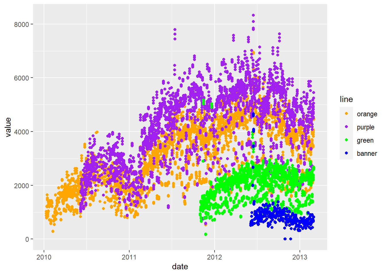

### Let's make Lines!
g + geom_line()

### let's make a new plot of points
gpoint <- g + geom_point()
### let's plot the value by the type of value - boardings/average, etc
gpoint + facet_wrap(~ type)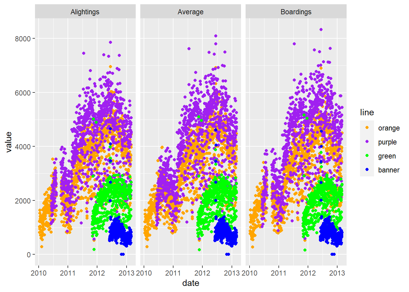

OK let’s turn off some warnings - making warning=FALSE (in knitr) as an option.

## let's compare vertically 
gpoint + facet_wrap(~ type, ncol=1)

gfacet = g + facet_wrap(~ type, ncol=1)

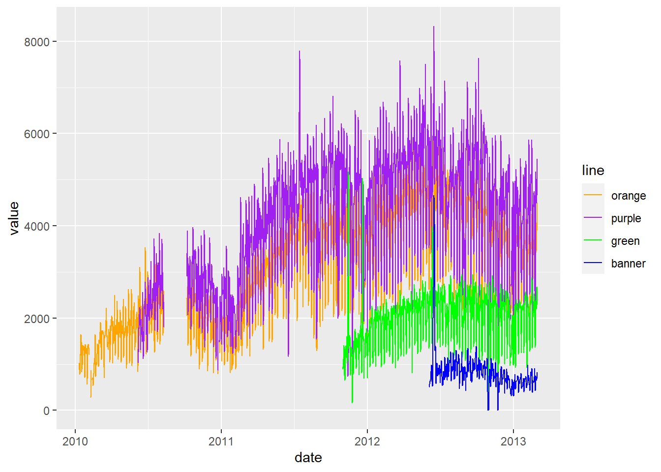
We can also smooth the data to give us a overall idea of how the average changes over time. I don’t want to do a standard error (se).

## let's smooth this - get a rough estimate of what's going on
gfacet + geom_smooth(se=FALSE)

`geom_smooth()` using method = 'gam' and formula = 'y ~ s(x, bs =
"cs")'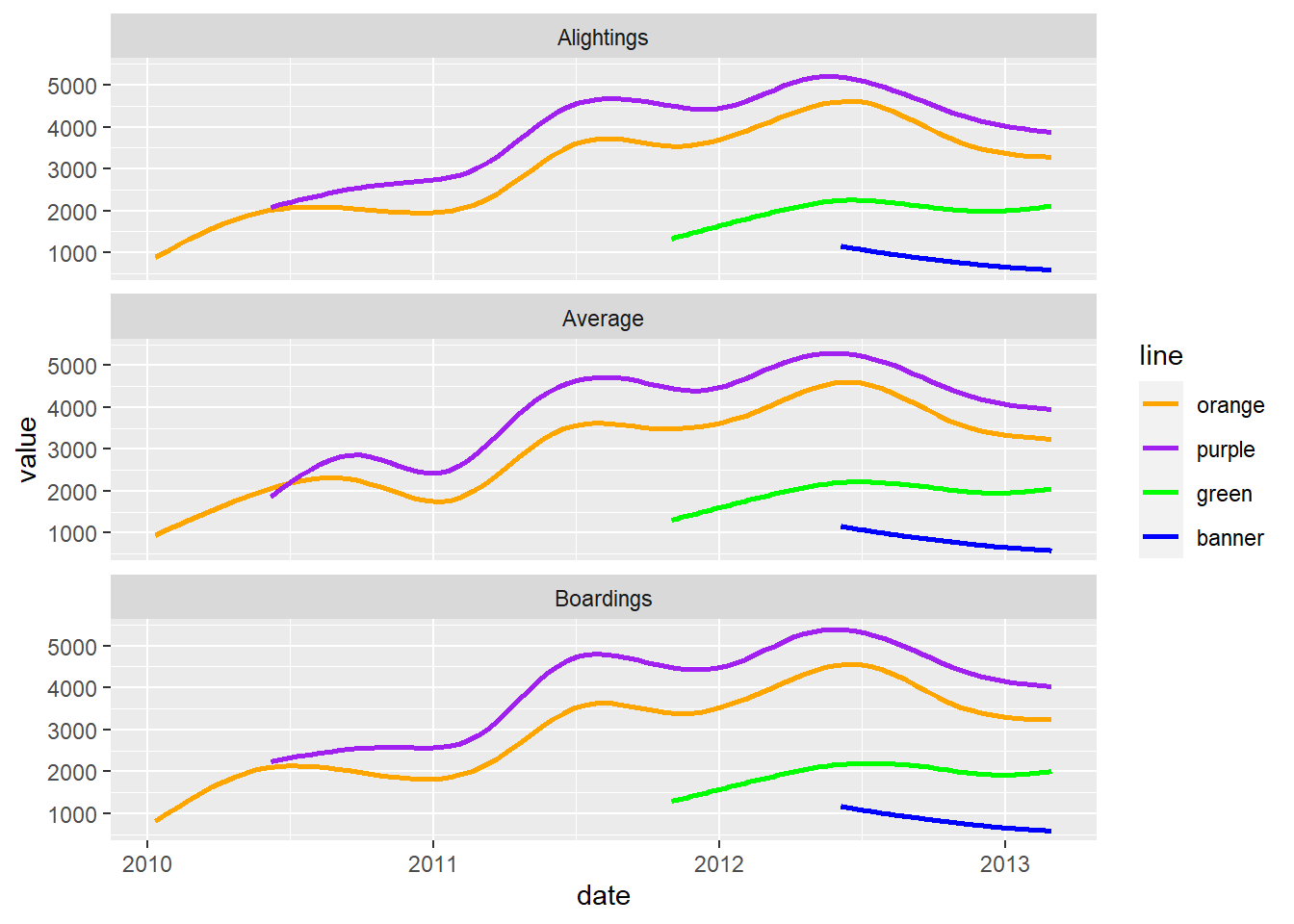

OK, I’ve seen enough code, let’s turn that off, using echo=FALSE.

`geom_smooth()` using method = 'gam' and formula = 'y ~ s(x, bs =
"cs")'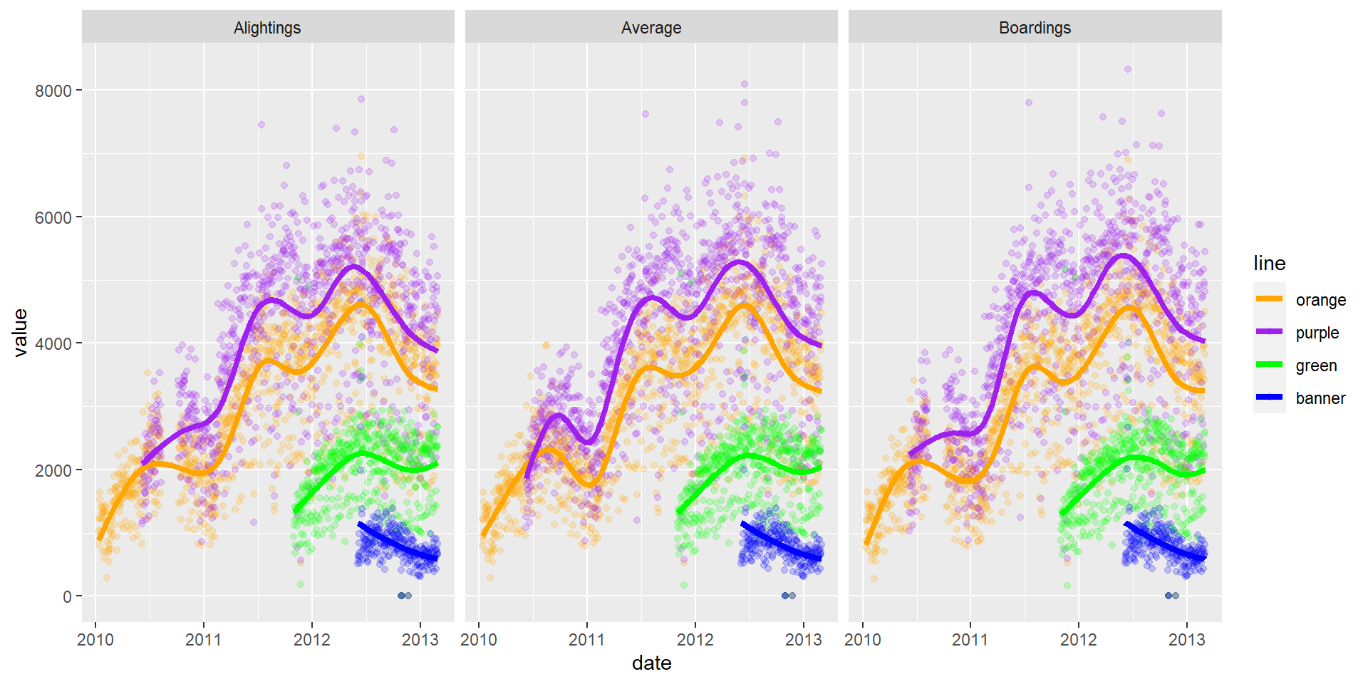

There are still messages, but we can turn these off with message = FALSE