Assessing the Model Assumptions

MLR Model Assumptions

The four conditions (LINE) that comprise the multiple linear regression model are

• The mean of the response at each value of the predictor, \(x_i\), is a Linear function of the \(x_i\).
• The errors, \(\varepsilon_i\), are Independent.
• The errors, \(\varepsilon_i\), are Normally distributed.
• The errors, \(\varepsilon_i\), have Equal variances.

In multiple linear regression, we can assess these assumptions by examining the errors ,\(e_i=\y_i-\hat{y}_i\). An equivalent way to state these four assumptions in terms of the errors, is that the true errors, \(\varepsilon_i\), are independent and have a normal distribution with mean 0 and constant variance.

The independence assumption has to be verified based on the subjects, and how the data was collected. Is is reasonable to beleive that the responses (or error) of one subject is independent of anothers? When this is not true, we will need to include these correlations in our model. This is the subject of mixed models, that we will discuss later.

Assessing the Linearity Assumptions

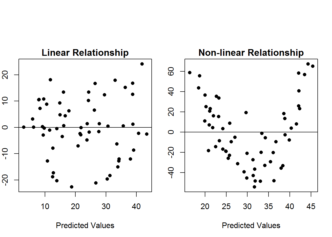
If the relationship between the predictors and the mean response is (approximately) linear, then the errors should have mean 0. We can check this assumption by examining a plot of residuals vs the predicted values (\(e_i\) vs \(y_i\)). If the linearity assumption is met, the resulting scatterplot should not show any trend. It should look like a cloud of points centered around the horizontal line \(y=0\). This means the vertical average of the points remains close to zero as we move from left to right.

Below are some example scatterplot of residuals vs predicted values. The scatterplot on the left shows no clear patter. We just see random scatter above and below the line \(y=0\), but in the second plot, there is a clear curved (quadratic) pattern. This second indicates that the linear assumption is not met, and we need to rethink out model or use another technique.

• To address the linearity assumption, we could add other terms into model, e.g. consider a quadratic model or we could transform the predictors or response.

Assessing the Normally Distributed Errors Assumption

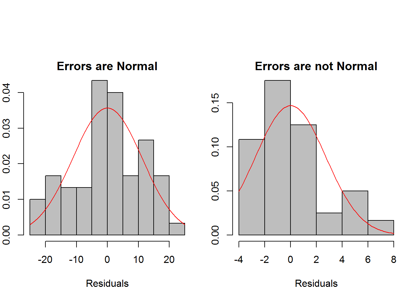
This assumption is usually assessed with histograms and qq plots. In histograms, we want to see a symmetric and bell shaped distribution. We can also an estimated normal density curve to the histogram to help asses whether the histogram looks normal or not. Do note that with small samples, it is unlikely that we will see a bell shaped histogram even if the data did truly come from a normal distribution. In this case, we are looking to see that there are no major deviations from normality such as heavy skewness or outliers. We can see in the first histogram, that the histogram looks symmetric and bell shapes, showing no major deviations from the normal distribution, but in the second histogram, the errors are heavily right skewed.

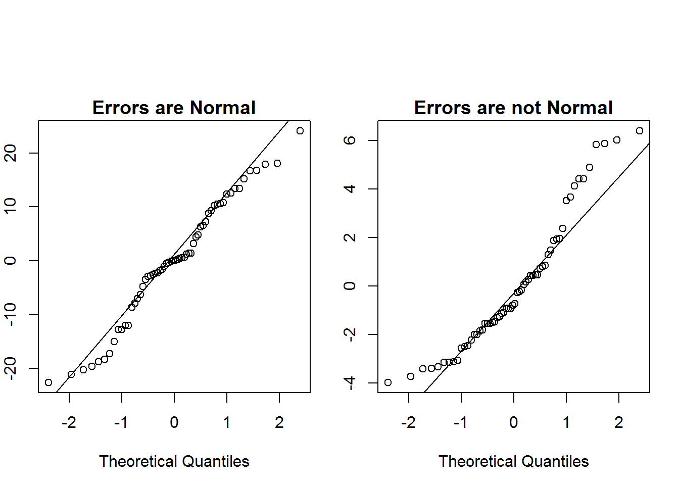
We can also use QQ plots to check the normal assumptions. Again, we are more concerned with major deviations from normality, than the data perfectly following the line in the QQ plot. We can see in the QQ plot on the left that the residuals roughly follow a normal distribution, but the errors in the plot on the right greatly deviate from the line near the tails indicating heavy skewness.

Assessing the Equal Variance Assumption

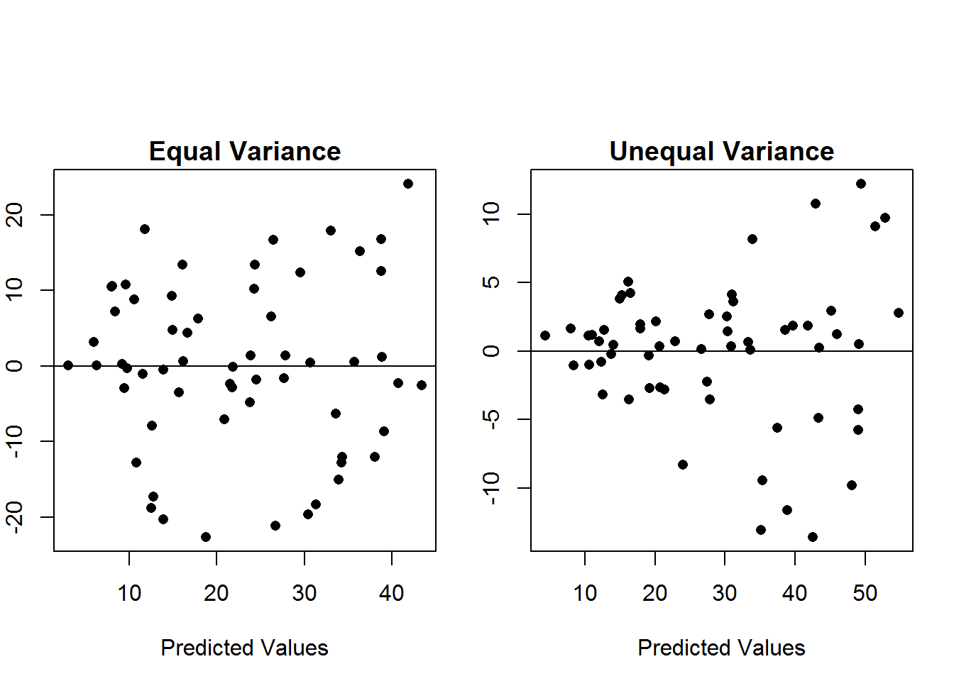
For the equal variance assumption, we should examine a plot of the residuals vs the predicted values. If the variance is constant, then the vertical spread should remain constant. We should not see any “fanning” out of the residuals. In the left scatterplot, we see an example where the equal variance assumption is met. The random scatter above and below the line y=0 remains roughly constant in terms of spread above and below the line. However, in the the scatterplot on the right, we see an example of unequal variances. As you move from left to right in the plot, the vertical spread is increasing.

Possible methods to address unequal variances:

• Common transformations to try to fix the unequal variances are log and square root transforms of the response.
• Weighted least squares can alos be used.

Why Are the Assumptions Important

The model assumptions are important for inference. If the model assumptions are not met then our results will not be valids since

• The regression parameters will be biased if the linearity assumption is not met
• Standard errors will be wrong if the normal errors, equal variance, or independence assumptions are not met leading to incorrect confidence intervals and p-values.

Other Problems in Regression

There are some other potential issues that affect the reliability of our regression estimates.

1. Outliers
   • This is a point for which the y-value is unusual (far away from the rest of the data). Outliers can have a large effect on both estimates of the slope parameters and their standard errors. If this data point was an error, such as a typo or from a different population than the one we are interested in, then it can be removed from the dataset. The outlier cannot be discarded unless it is an error. If it is not an error, then it may be very informative. We may be missing an important varaible in our model or have some other model inadequacy that needs to be addressed.
2. High Leverage Points
   • High leverage points are data points that have an unusual x-value. These points can have a similar impact as outliers. They can drastically change the estimated regression line. Again, these points should be examined for errors. If the points is found not to be an error, then we will need to consider a different model that can accomodate this points.
3. Collinearity
   • Collinearity refers to when two or more predictors are closely related to one another. In this case, these variables provide the same information about the response. This leads to unstable estimates of the regression parameters. These can be detected by looking at variance inflation factors. If predictors are identified as collinear, then there are two solutions: 1. We can drop one of them, since they are providing redundant information 2. We can combine in to a single variable.