EDA and Model Building
## Warning: package 'haven' was built under R version 3.4.1In this section, we will discuss some usefule plots for exploratory data analysis. These plots will help us decide on both the mean structure (fixed effects) and the variance structure (random effects and error structure). The dataset, we will use is from a study of therapeutic use of hormones. The study examined the effoct of the inhibition of tesstosterone production in male rates on their craniofacial growth. A total of 50 male rats were randomized to either control or one of two treament groups, where they either received low or high dose of Decapeptyl, which is an inhibitor of testosterone production in rats. The treatment was started at the age of 45 days and measurements were taken every 10 days for a total of 7 measurements.The response measured is the height of the skull measured in pixels from X-rays.
Investigating the Mean Structure
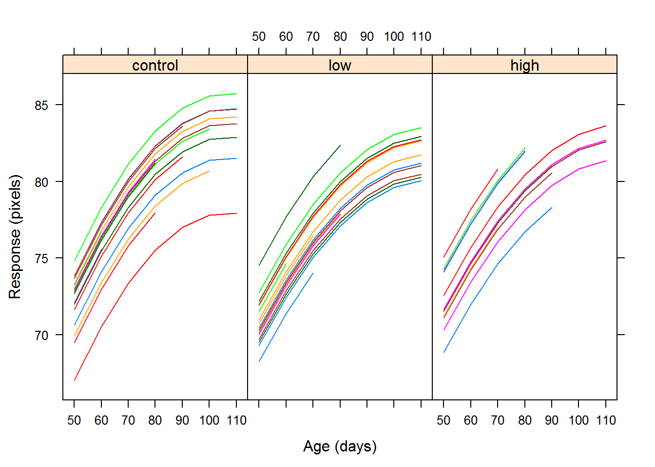
The first plot is called a profile plot, where we examine the response against a coviariate for each individual subject.
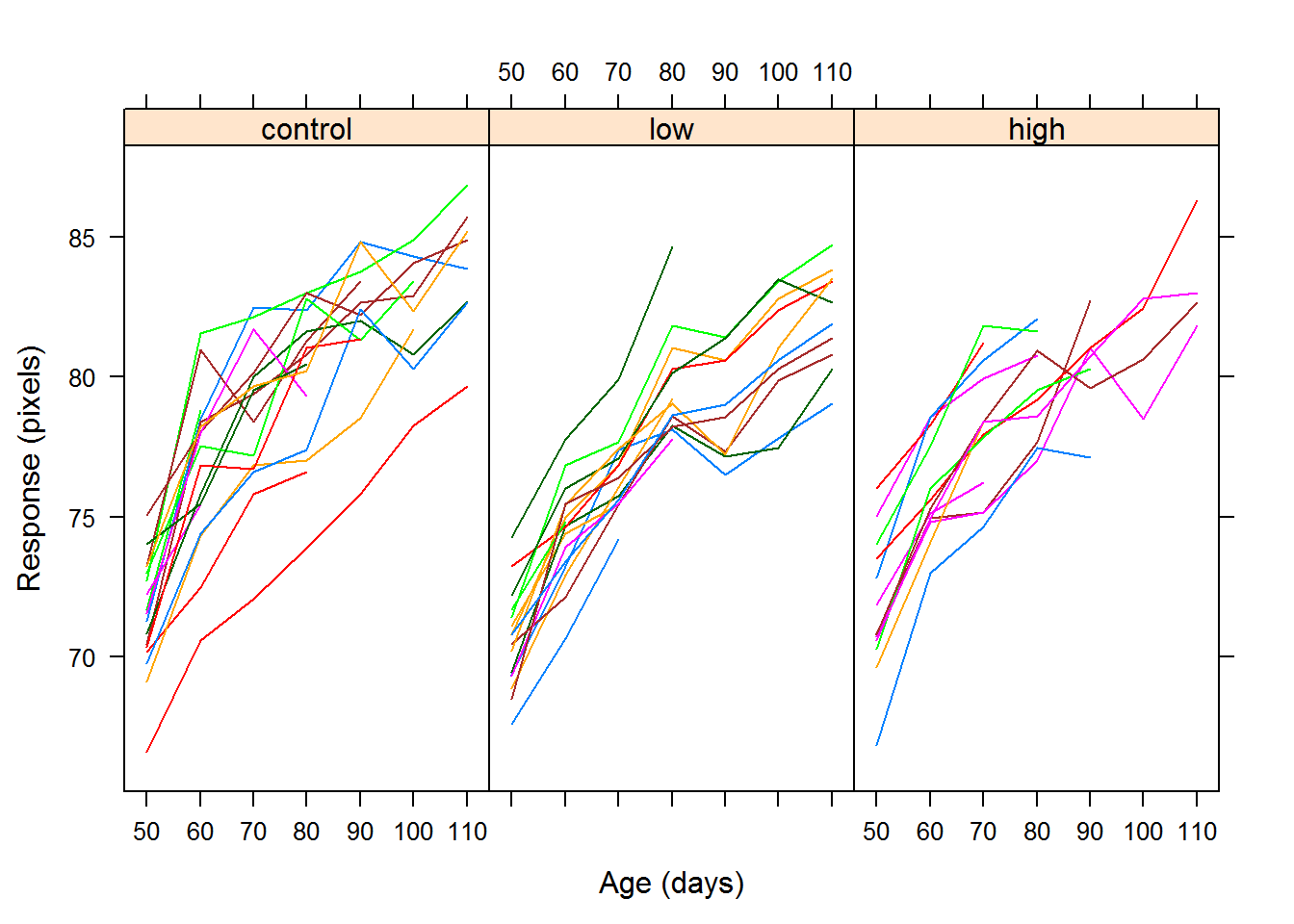
The following plots are scatterplots of the repsonse versus time for each treatment group with a lowess curve for the mean response over time. The profile appears to be curved, so we may want to try a quadratic model in time.
## Warning in plot.window(...): "data" is not a graphical parameter## Warning in plot.window(...): "subset" is not a graphical parameter## Warning in plot.xy(xy, type, ...): "data" is not a graphical parameter## Warning in plot.xy(xy, type, ...): "subset" is not a graphical parameter## Warning in axis(side = side, at = at, labels = labels, ...): "data" is not
## a graphical parameter## Warning in axis(side = side, at = at, labels = labels, ...): "subset" is
## not a graphical parameter## Warning in axis(side = side, at = at, labels = labels, ...): "data" is not
## a graphical parameter## Warning in axis(side = side, at = at, labels = labels, ...): "subset" is
## not a graphical parameter## Warning in box(...): "data" is not a graphical parameter## Warning in box(...): "subset" is not a graphical parameter## Warning in title(...): "data" is not a graphical parameter## Warning in title(...): "subset" is not a graphical parameter## Warning in plot.window(...): "data" is not a graphical parameter## Warning in plot.window(...): "subset" is not a graphical parameter## Warning in plot.xy(xy, type, ...): "data" is not a graphical parameter## Warning in plot.xy(xy, type, ...): "subset" is not a graphical parameter## Warning in axis(side = side, at = at, labels = labels, ...): "data" is not
## a graphical parameter## Warning in axis(side = side, at = at, labels = labels, ...): "subset" is
## not a graphical parameter## Warning in axis(side = side, at = at, labels = labels, ...): "data" is not
## a graphical parameter## Warning in axis(side = side, at = at, labels = labels, ...): "subset" is
## not a graphical parameter## Warning in box(...): "data" is not a graphical parameter## Warning in box(...): "subset" is not a graphical parameter## Warning in title(...): "data" is not a graphical parameter## Warning in title(...): "subset" is not a graphical parameter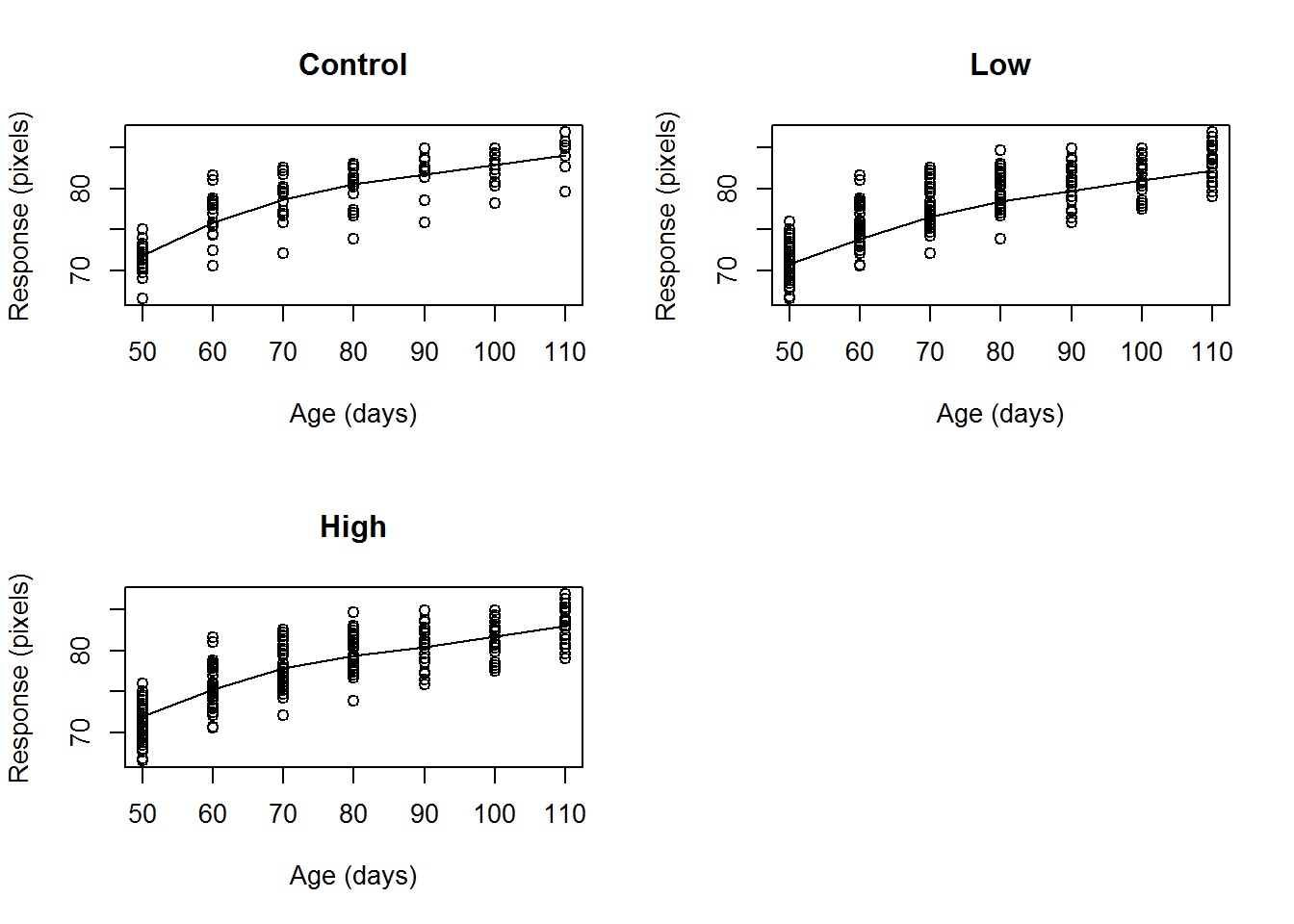 Other methods of visualized the mean relationship include boxplots over time and series plots of the mean at each time point. One way to assess the fit of the chosen mean structure is to fit this linear regression model with the chosen mean struture to each subject. From each fit, you will have an \(R^2\). A plot of the \(R_i^2\) versus the number of measurements on each subject can help compare mean structures. The more \(R^2_i\) that are high the better the fit.
Investigating the Random Effects Structure
Once we have chosen a mean structure, we can examine the residuals from an ordinary least squares fit using the chosen mean structure. Let’s plot the squared residuals vs time.
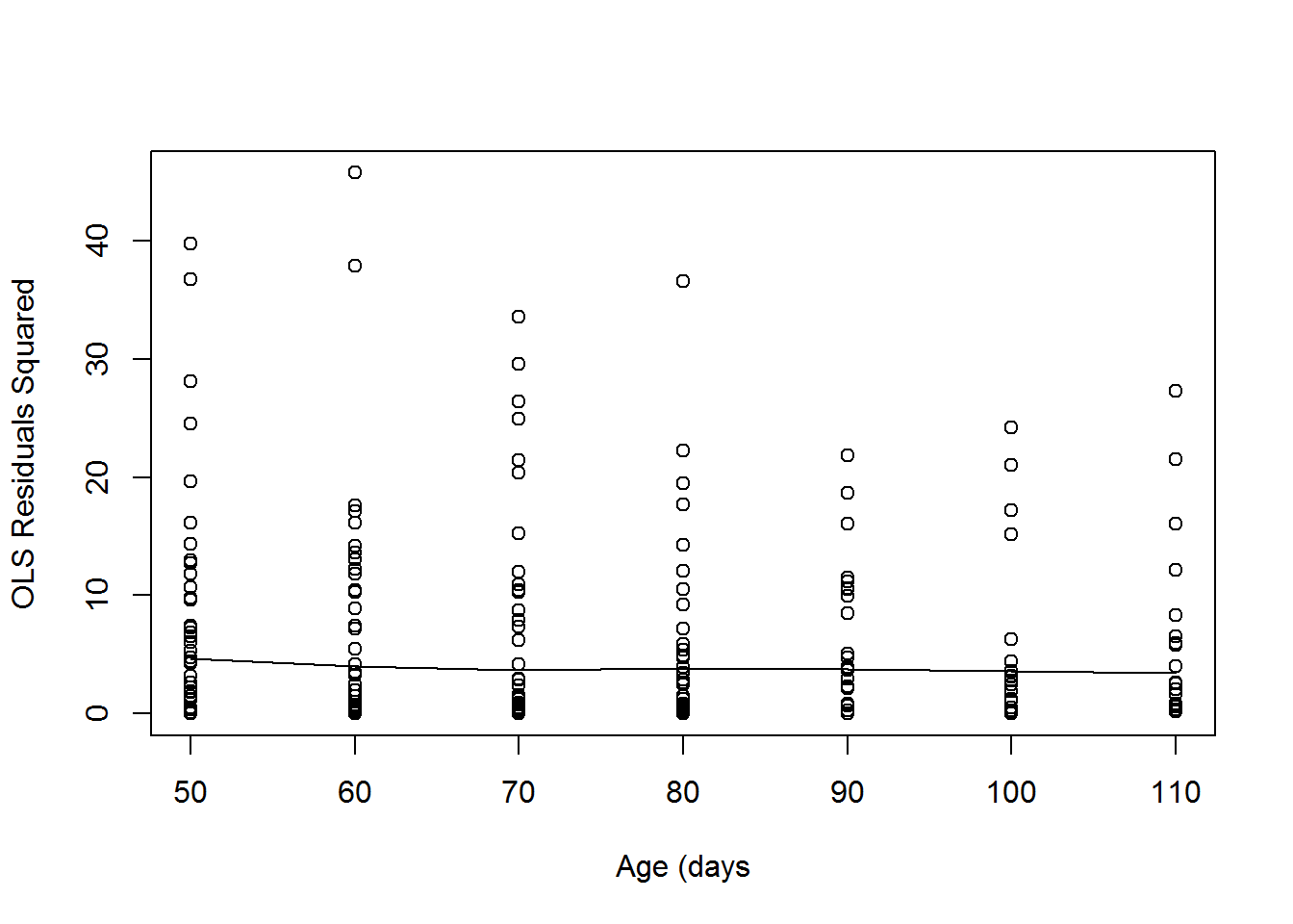
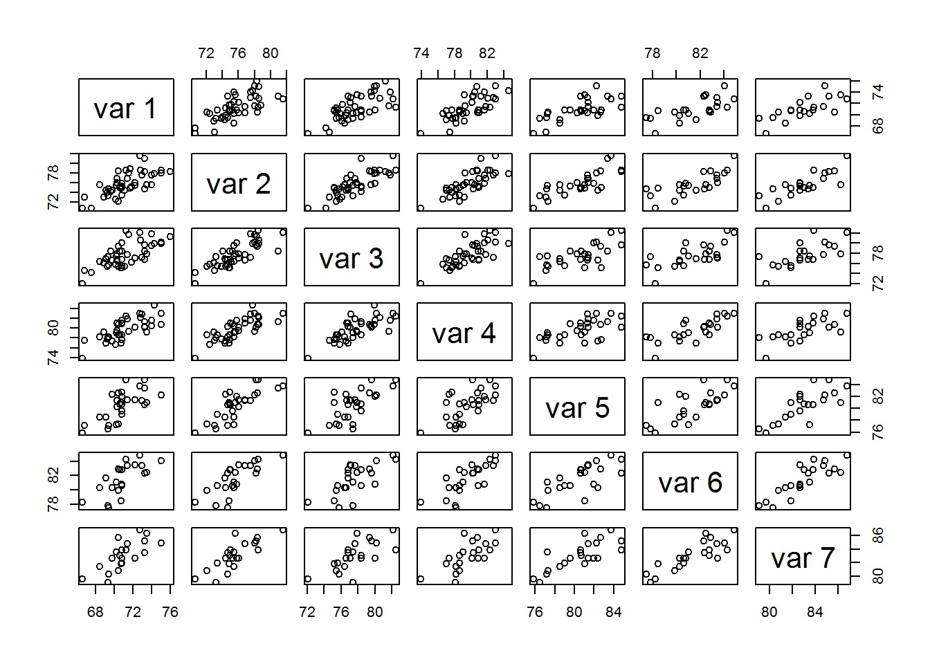
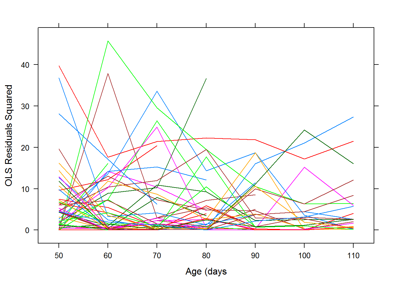 In this case, the variance function looks linear with a slight decrease, so a random intercept and slope model might be enough for this data. This also agrees with the profile plot of the residuals. We can test later to see if the random slope is needed. Another check of this would be to look at the scatterplot matrix. A random intercept model assumes that the variance is constant over time.
- In general, trying to find a function of the residuals squared vs the
## Loading required package: Matrix## Warning: Some predictor variables are on very different scales: consider
## rescaling
## Warning: Some predictor variables are on very different scales: consider
## rescaling## refitting model(s) with ML (instead of REML)## Data: rats.dat
## Models:
## rats.mod2: RESPONSE ~ TIME * GROUP + I(TIME^2) * GROUP + (1 | SUBJECT)
## rats.mod: RESPONSE ~ TIME * GROUP + I(TIME^2) * GROUP + (1 + TIME | SUBJECT)
## Df AIC BIC logLik deviance Chisq Chi Df Pr(>Chisq)
## rats.mod2 11 971.54 1010.4 -474.77 949.54
## rats.mod 13 975.54 1021.4 -474.77 949.54 0.0011 2 0.9994## Linear mixed model fit by REML ['lmerMod']
## Formula: RESPONSE ~ TIME * GROUP + I(TIME^2) * GROUP + (1 | SUBJECT)
## Data: rats.dat
##
## REML criterion at convergence: 1012.9
##
## Scaled residuals:
## Min 1Q Median 3Q Max
## -2.39030 -0.64236 0.01634 0.59340 2.95946
##
## Random effects:
## Groups Name Variance Std.Dev.
## SUBJECT (Intercept) 3.509 1.873
## Residual 1.644 1.282
## Number of obs: 252, groups: SUBJECT, 50
##
## Fixed effects:
## Estimate Std. Error t value
## (Intercept) 44.5939813 2.3846704 18.700
## TIME 0.7175971 0.0629588 11.398
## GROUPlow 2.4757256 3.3797078 0.733
## GROUPhigh 4.0422830 3.7172364 1.087
## I(TIME^2) -0.0033519 0.0004017 -8.344
## TIME:GROUPlow -0.1057914 0.0887624 -1.192
## TIME:GROUPhigh -0.1194817 0.0994383 -1.202
## GROUPlow:I(TIME^2) 0.0006470 0.0005626 1.150
## GROUPhigh:I(TIME^2) 0.0007636 0.0006432 1.187
##
## Correlation of Fixed Effects:
## (Intr) TIME GROUPl GROUPh I(TIME TIME:GROUPl
## TIME -0.975
## GROUPlow -0.706 0.688
## GROUPhigh -0.642 0.625 0.453
## I(TIME^2) 0.955 -0.993 -0.674 -0.613
## TIME:GROUPl 0.691 -0.709 -0.974 -0.443 0.704
## TIME:GROUPh 0.617 -0.633 -0.435 -0.976 0.629 0.449
## GROUPl:I(TIME^2) -0.682 0.709 0.955 0.437 -0.714 -0.993
## GROUPh:I(TIME^2) -0.596 0.620 0.421 0.955 -0.625 -0.440
## TIME:GROUPh GROUPl:I(TIME^2)
## TIME
## GROUPlow
## GROUPhigh
## I(TIME^2)
## TIME:GROUPl
## TIME:GROUPh
## GROUPl:I(TIME^2) -0.449
## GROUPh:I(TIME^2) -0.992 0.446
## fit warnings:
## Some predictor variables are on very different scales: consider rescaling## Groups Name Std.Dev.
## SUBJECT (Intercept) 1.8732
## Residual 1.2822The random slope is not significant, so we go with just the random intercept. For this model, the variance function is
\[\sigma^2_u+\sigma^2_e=3.509+1.644=5.153\]
 There may still be some residual covariance that we need to model with serial correlation such as autrogressive structures for the residual variance. We will not cover this topic here, but you can read about it in the references provided in the syllabus.
Here are the prediction lines for the fitted random intercept model.