Adding a Level 2 Variable
So far we have considered explanatory variables defined at the lowest level of the hierarchical structure. For example, in our analysis of the correlates of birth weights, we have included individual characteristics such as mother’s age at time of birth. The multilevel models we have considered up to this point control for clustering, and allow us to quantify the extent of dependency and to investigate whether the effects of level 1 variables vary across these clusters. One particular benefit of multilevel modelling, however, is the ability to explore the effects of group-level variables while simultaneously allowing for the possibility that y may be influenced by unmeasured group factors. Variables defined at level 2 are often called contextual variables and their effects on an individual’s y-value are called contextual effects.
If contextual effects are of interest, it is particularly important to use a multilevel modelling approach because the standard errors of coefficients of level 2 variables may be severely underestimated when a single-level model is used.
Examples of research questions involving contextual effects include:
- What are the pathways through which income affects individual health outcomes? Do people with a low income have poor health because their material living standards are lower than those with higher incomes? For example, having a low income may be associated with a low standard of housing or poor diet. Or does the relationship work at an area (macro) level? According to the relative income hypothesis, a person’s income relative to that of their neighbours is an important determinant of health which operates over and above any micro effects. Thus an individual with a low income living in a society with large income inequalities would be expected to have poorer health than someone with the same income but living in a more egalitarian society. To test the relative income hypothesis, we could include in our model an aggregate measure of income inequality. For example, in a study of variations in health for individuals (level 1) in countries (level 2) we might include the within-country standard deviation of income or the Gini coefficient.
- What is the role of family background on child health? Suppose we have health measures on all children (level 1) in a family (level 2). We might first calculate the proportion of the total variance in health that is attributable to differences between families (the variance partition coefficient or intra-family correlation). We could then investigate whether any between-family variation can be explained by family characteristics, shared by all children in the family, such as household socio-economic status, parental education and lifestyle factors.
A level 2 explanatory variable can be included in a multilevel model in exactly the same way as a level 1 variable. For example, if we have a level 1 variable \(x_{1ij}\) and a level 2 variable \(x_{2i}\), then the random intercept model becomes:
\[y_{ij}=\beta_0+\beta_1x_{1ij}+\beta_2x_{2i}+u_{i}+\varepsilon_{ij}.\]
(Note that a level 2 variable does not have an j subscript because, by definition, its values do not vary from individual to individual within a level 2 unit.)
We can think of this model hierachically as:
- Level 1: \(y_{ij}=\beta_{0i}+\beta_{1}x_{1ij}+\varepsilon_{ij}\)
- Level 2: \(\beta_{0i}=\beta_0+\beta_2x_{2i}+u_i\)
Since the level 2 variable does not vary at the individual level, its value is fixed for a specific group. In this case, we are using the group level variable to adjust the subject specific intercepts (baseline effect).
Contextual variables may come from a number of sources. Data may be collected at level 2, e.g. community surveys in which key figures in the community are interviewed, or data from geographical information systems (GIS) on the location of health facilities. Contextual data may also derive from level 1 data that is aggregated to form level 2 variables. These data may come from an external source, e.g. a Census, or the same source as the level 1 data to be analysed.
If the contextual variable is the level 2 mean of a level 1 variable that is also included in the model becomes
\[y_{ij}=\beta_0+\beta_1x_{ij}+\beta_2\bar{x}_{i}+u_{i}+\varepsilon_{ij}.\] where \(\bar{x}_i\) is the mean of x in group i.
In the model above, \(\beta_1\) is the within-group effect of x and \(\beta_1+\beta_2\) is the between-group effect of x. The within-group coefficient measures the relationship between an individual’s x and y values within a group. The between-group effect measures the relationship between x and y at the group level, i.e. the effect of the group mean of x on the group mean of y . \(\beta_2\) is the contextual effect of x, which is the effect of the group mean of x on an individual y that is over and above the effect of an individual x on y.
So that the within-group and between-group effects can each be represented by a single parameter, the model above can be conveniently re-expressed as
\[y_{ij}=\beta_0+\beta_1^\star (x_{ij}-\bar{x}_i)+\beta_2^\star \bar{x}_{i}+u_{i}+\varepsilon_{ij}\]
where \(\beta_1^\star=\beta_1\) is the within group effect, and \(\beta_2^\star=\beta_1+\beta_2\) is the between group effect. These two models are equivalent, but the latter model produces a direct estimate and standard error for the between group effect.
The transformation of \(x_{ij}\) to \(x_{ij}-\bar{x}_i\) is called group mean centering, as opposed to grand mean centering.
Example: Within and between mother relationships between birth weight and mother’s age
Let’s consider the relationship between an individual’s birth weight and mother’s age and mother’s average age at birth over the five children. Mother i’s age during the birth of infant j (\(x_{ij}\)) is measured in years and the average mother’s age (\(\bar{x}_j\)) is the average of the mother’s age at the birth’s of her five children. The following table gives the results of three models.
- Model 1: only includes the individual mother’s age at birth (\(x_{ij}\)) as a predictor
- Model 2: includes both the individual age (\(x_{ij}\)) and the mother’s average age (\(\bar{x}_i\)) as predictors
- Model 3: includes both the group mean centered mohter’s age (\(x_{ij}-\bar{x}_i\)) and the mother’s average age (\(\bar{x}_i\)) as predictors
## Linear mixed model fit by maximum likelihood  ['lmerMod']
## Formula: bweight ~ momage + (1 | momid)
##    Data: gababies.dat
##
##      AIC      BIC   logLik deviance df.resid
##  15332.7  15352.3  -7662.3  15324.7      996
##
## Scaled residuals:
##     Min      1Q  Median      3Q     Max
## -5.1170 -0.4428  0.0475  0.5290  4.0915
##
## Random effects:
##  Groups   Name        Variance Std.Dev.
##  momid    (Intercept) 126825   356.1
##  Residual             198850   445.9
## Number of obs: 1000, groups:  momid, 200
##
## Fixed effects:
##             Estimate Std. Error t value
## (Intercept) 2793.576     72.934    38.3
## momage        15.804      3.096     5.1
##
## Correlation of Fixed Effects:
##        (Intr)
## momage -0.918
## Linear mixed model fit by maximum likelihood ['lmerMod']
## Formula: bweight ~ momage + momageGC + (1 | momid)
## Data: gababies.dat
##
## AIC BIC logLik deviance df.resid
## 15334.1 15358.6 -7662.1 15324.1 995
##
## Scaled residuals:
## Min 1Q Median 3Q Max
## -5.1358 -0.4431 0.0506 0.5373 3.9339
##
## Random effects:
## Groups Name Variance Std.Dev.
## momid (Intercept) 126459 355.6
## Residual 198821 445.9
## Number of obs: 1000, groups: momid, 200
##
## Fixed effects:
## Estimate Std. Error t value
## (Intercept) 2694.799 150.482 17.908
## momage 14.625 3.473 4.211
## momageGC 5.745 7.660 0.750
##
## Correlation of Fixed Effects:
## (Intr) momage
## momage 0.000
## momageGC -0.875 -0.453## Linear mixed model fit by maximum likelihood ['lmerMod']
## Formula: bweight ~ I(momage - momageGC) + momageGC + (1 | momid)
## Data: gababies.dat
##
## AIC BIC logLik deviance df.resid
## 15334.1 15358.6 -7662.1 15324.1 995
##
## Scaled residuals:
## Min 1Q Median 3Q Max
## -5.1358 -0.4431 0.0506 0.5373 3.9339
##
## Random effects:
## Groups Name Variance Std.Dev.
## momid (Intercept) 126459 355.6
## Residual 198821 445.9
## Number of obs: 1000, groups: momid, 200
##
## Fixed effects:
## Estimate Std. Error t value
## (Intercept) 2694.799 150.482 17.908
## I(momage - momageGC) 14.625 3.473 4.211
## momageGC 20.370 6.827 2.984
##
## Correlation of Fixed Effects:
## (Intr) I(-mGC
## I(mm-mmgGC) 0.000
## momageGC -0.981 0.000| Model 1 | Model 2 | Model 3 | ||||
|---|---|---|---|---|---|---|
| Variable | Est. | SE | Est. | SE | Est. | SE |
| Fixed Part | ||||||
| Constant | 2794 | 72.9 | 2695 | 150.5 | 2695 | 150.5 |
| xij | 15.8 | 3.10 | 14.625 | 3.5 | - | - |
| xij - xi | - | - | - | - | 14.6 | 3.5 |
| xi | - | - | 5.745 | 7.7 | 20.37 | 6.8 |
| Random Part | ||||||
| σ2u | 126825 | - | 126459 | - | 126459 | - |
| σ2e | 198850 | - | 198821 | - | 198821 | - |
- From model 1, we can conclude that there is a significant, positive relationship between the mother’s age at birth and the infant’s birth weight. Each 1 year increase in mother’s age is associated with a mean increase of 15.8 grams in birth weight.
- Recall that models 2 and 3 are equivalent and the coefficient of \(x_{ij}\) (or equivalently the coefficient of \(x_{ij}-\bar{x}_i\)) is interepreted as the within mother association between mother’s age and birth weight.
- The between mother association between birth weight and mother’s age is represented by \(20.37=14.625+5.745\). We therefore conclude that, for a given mother, a higher age at birth is associated with a higher birth weight. However, the larger between mother effect (\(\bar{x}_i\) coefficient$) suggests that the relationship between age and birth weight is stronger at the mother level.
- The contextual effect of age is the coefficient of of \(\bar{x}_i\) in model 2 which is estimated to be 5.745, but with a standard error of 7.7, it is not significant. Had it been significant, we could have concluded that, over and above the individual association, there is a contextual association: an individual infant with a mother at a given age will, on average, have a higher birth weight if he or she has a mother with a higher average age at births.
- The addition of the of mother level age reduces the mother level varaince from 126825 to 126549, and so explains \((126825-126549)/126825=0.22\%\) of the between mother variance.
Cross-level interactions
As in multiple regression, we can allow for the possibility that the effect of one explanatory variable on y depends on the value of another explanatory variable. Recall that such effects are called interaction effects and are represented in a model by including the product of the interacting variables as explanatory variables. Interactions can also be included in a multilevel model and these can be between any pair (or larger set) of variables, regardless of the level at which they are defined. An interaction between a level 1 variable and a level 2 variable is known as a cross-level interaction.
Example: Are gender differences in birth weight related to a mother’s average age at birth?
One question we may ask with the birth weight data is do male infants have higher birth weights for mother’s with a higher average age at births? To answer this question we will examine the following model:
\[y_{ij}=\beta_0+\beta_1x_{1ij}+\beta_2\bar{x}_{2i} + \beta_3x_{1ij}*\bar{x}_{2i}+u_{0i}+u_{1i}x_{1ij}+\beta_4(x_{2ij}-\bar{x}_{2i})+\varepsilon_{ij}\]
where
- \(x_{1ij}=\text{ the gender of infant j from mother i}\), where it takes the value 1 for male and 0 for female$
- \(x_{2ij}=\text{ the age of mother i at the birth of infant j}\)
- \(\bar{x}_{2i}=\text{ the mean age at births of the five children for mother i}\)
Notice that we have a cross-level effect between gender and the group mean age of the mother at birth. A significant interaction term would mean that the gender effect on birth weight depends on the mother’s mean age at birthing. Below is the output and a summary table for the model above (model 2) and the model without the interaction term (model 1).
## Linear mixed model fit by maximum likelihood  ['lmerMod']
## Formula:
## bweight ~ gender + momageGC + I(momage - momageGC) + (1 + gender |
##     momid)
##    Data: gababies.dat
##
##      AIC      BIC   logLik deviance df.resid
##  15333.7  15372.9  -7658.8  15317.7      992
##
## Scaled residuals:
##     Min      1Q  Median      3Q     Max
## -5.3041 -0.4486  0.0467  0.5201  4.1677
##
## Random effects:
##  Groups   Name        Variance Std.Dev. Corr
##  momid    (Intercept) 159610   399.5
##           gendermale   27826   166.8    -0.57
##  Residual             191233   437.3
## Number of obs: 1000, groups:  momid, 200
##
## Fixed effects:
##                      Estimate Std. Error t value
## (Intercept)          2692.450    151.724  17.746
## gendermale             38.666     32.434   1.192
## momageGC               19.515      6.811   2.865
## I(momage - momageGC)   14.341      3.435   4.175
##
## Correlation of Fixed Effects:
##             (Intr) gndrml momgGC
## gendermale  -0.152
## momageGC    -0.973  0.017
## I(mm-mmgGC)  0.002  0.038 -0.006
## (Intercept) gendermale
## (Intercept) 159610.38 -38088.88
## gendermale -38088.88 27826.14
## attr(,"stddev")
## (Intercept) gendermale
## 399.5127 166.8117
## attr(,"correlation")
## (Intercept) gendermale
## (Intercept) 1.0000000 -0.5715328
## gendermale -0.5715328 1.0000000## Linear mixed model fit by maximum likelihood ['lmerMod']
## Formula:
## bweight ~ gender * momageGC + I(momage - momageGC) + (1 + gender |
## momid)
## Data: gababies.dat
##
## AIC BIC logLik deviance df.resid
## 15334.2 15378.4 -7658.1 15316.2 991
##
## Scaled residuals:
## Min 1Q Median 3Q Max
## -5.2510 -0.4510 0.0485 0.5223 3.9613
##
## Random effects:
## Groups Name Variance Std.Dev. Corr
## momid (Intercept) 159146 398.9
## gendermale 26325 162.2 -0.58
## Residual 191220 437.3
## Number of obs: 1000, groups: momid, 200
##
## Fixed effects:
## Estimate Std. Error t value
## (Intercept) 2570.699 181.840 14.137
## gendermale 238.394 167.392 1.424
## momageGC 25.101 8.219 3.054
## I(momage - momageGC) 14.557 3.437 4.236
## gendermale:momageGC -9.209 7.573 -1.216
##
## Correlation of Fixed Effects:
## (Intr) gndrml momgGC I(-mGC
## gendermale -0.566
## momageGC -0.981 0.552
## I(mm-mmgGC) -0.025 0.054 0.021
## gndrml:mmGC 0.551 -0.981 -0.560 -0.047## (Intercept) gendermale
## (Intercept) 159146.44 -37236.89
## gendermale -37236.89 26324.61
## attr(,"stddev")
## (Intercept) gendermale
## 398.9316 162.2486
## attr(,"correlation")
## (Intercept) gendermale
## (Intercept) 1.0000000 -0.5752993
## gendermale -0.5752993 1.0000000| Model 1 | Model 2 | |||
|---|---|---|---|---|
| Variable | Est. | SE | Est. | SE |
| Fixed Part | ||||
| Intercept | 2692 | 152 | 2571 | 182 |
| Male | 38.7 | 32.5 | 238.4 | 167.4 |
| Individual minus mom mean age | 14.34 | 3.44 | 14.56 | 3.44 |
| Mom mean age | 19.52 | 8.81 | 25.10 | 8.22 |
| Mom mean age * Male interaction | - | - | -9.209 | 7.573 |
| Random part | ||||
| σ2u0 (intercept variance) | 159610 | - | 159146 | - |
| σ2u1 (female-male variance) | 27826 | - | 26326 | - |
| σu01 (covariance) | -38089 | - | -37237 | - |
| σ2e | 191233 | 191220 | - | |
The coefficient of the interaction variable in model 2 is not significant, but if it were, since it is negative and the male effect is positive, this would imply that the gender difference in birth weights decreases as the mean age at birth increases. Allowing the interaction between the mother’s average age at birth and the gender reduced the between mother variation in gender gender effect from 27826 to 26326. We can also explore the between mother variation in birth weights for males and females.
Model 1
- Female: 159610
- Male: \(159610+27826+2(-38089)=111258\)
Model 2
- Female: 159146
- Male: \(159146+26326+2*(-37237)=110998\)
Thus allowing for the cross-level interarction slightly reduces the between mother variance for both men and women, but mother effects remain stronger in men (higher variance).
Now, let’s graphically look at the gender differences in birth weights by mean age. The predicted birth weights are based on model 2 with the deviation between a mother’s age at birth and the mother’s mean age set to 0 and \(u_{0i}=u_{1j}=0\). That is, we are picturing the mean birth weight across all groups (the grand mean) for different mean ages at birth.
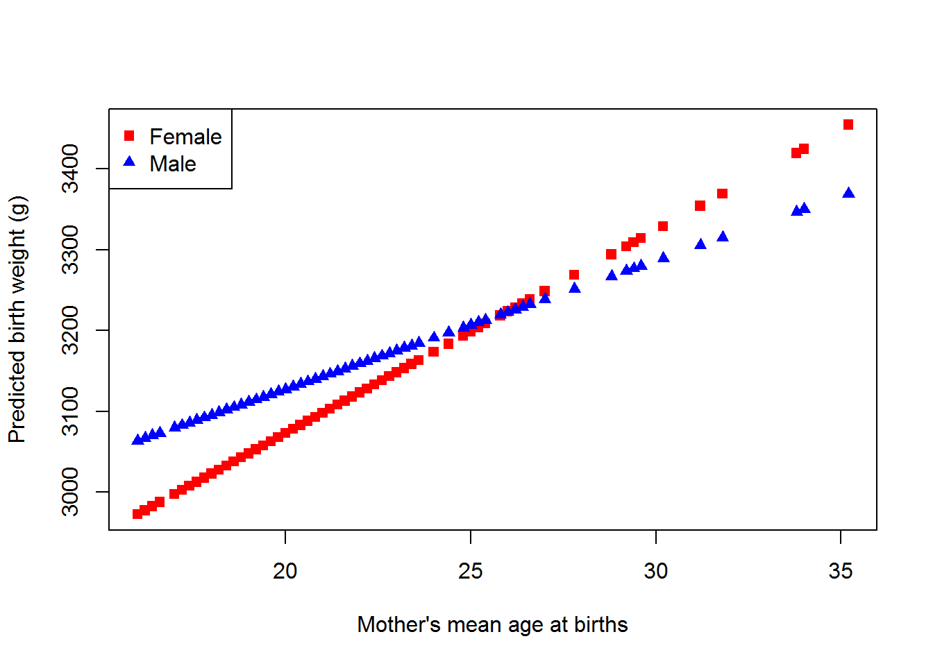
What we see in the plot is that for mother’s with lower mean ages males tend to have higher birth weights than females, but as the mean age increases, the difference in birth weight decreases until after about a mean age of 25 years old. Then females tend to weigh more than males and this difference grows as the mean mother’s age increases.