Random Intercept Models
What is multilevel modeling?
In the social, medical and biological sciences multilevel or hierarchical structures are the norm. Examples include individuals nested within geographical areas or institutions (eg, schools or employers), and repeated observations over time on individuals. Other examples of hierarchical and non-hierarchical structures were given in the previous sections. When individuals form groups or clusters, we might expect that two randomly selected individuals from the same group will tend to be more alike than two individuals selected from different groups. For example, families in the same neighborhood may have similar features such as education, financial status and other characteristics that influence their access to health care. Because fo these neighborhood effects, we would expect families in the same neighborhood to be more alike than families from different neighborhoods. By a similar argument, measurements taken on the same individual at different occasions, eg, physical attributes or social attitudes, will tend to more highly correlated than two measurements from different individuals. Such dependencies can therefore be expected to arise and we need multilevel models – also known as hierarchical linear models, mixed models, random effects models and variance components models - to analyse data with a hierarchical structure. Throughout this module we refer to the lowest level of observation in the hierarchy (eg, patient or measurement on a given occasion) as level 1, and the group or cluster (e.g., physician or individual) as level 2.
our goal is still to fit a regression model, but the standard multiple linear regression model assumes that all measurements units are independent. Specifically, we assume that the residuals, \(\varepsilon\), are independent of one another. If data are grouped and we have not taken account of group effects in our regression model, the independence assumption will not hold. Ignoring the clustering leads to incorrect standard errors for the regression parameters. Consequently confidence intervals will be too narrow and p-values will be too small, which may in turn lead us to infer that a predictor has a ‘real’ effect on the outcome when in fact the effect could be ascribed to chance. Underestimation of standard errors is particularly severe for coefficients of predictors that are measured at the group level, e.g. gender of the physician. Correct standard errors will be estimated only if variation among groups is allowed for in the analysis, and multilevel modelling provides an efficient means of doing this.
Obtaining correct standard errors is just one reason for using multilevel modelling. If you are interested only in controlling for clustering, rather than exploring it, there are other methods that can be used. For example, survey methodologists have long recognised the consequences of ignoring clustering in the analysis of data from multistage designs and have developed methods to adjust standard errors for design effects. Another approach is to model the dependency between observations in the same group explicitly using a marginal model. Both methods yield correct standard errors, but treat clustering as a nuisance rather than something of substantive interest in its own right. Multilevel modelling enables researchers to investigate the nature of between-group variability, and the effects of group-level characteristics on individual outcomes. Some examples of research questions that can be explored using multilevel models are given below:
- Do health outcomes vary across areas? Are between-area variations in health explained by differences in access to health services? Is the amount of variation between areas different for rural and urban areas?
- Does the rate of physical growth vary across children? Does variability in the growth rate differ for boys and girls?
A multilevel model for group effects: Random intercept model
Let’s start with the simplest (single level) model for the mean: a model for the mean with no dependent variables.
\[y_i=\beta_0+\varepsilon_i\]
where
- \(y_i\) is the value of \(y\) for the ith individual (\(i=1,\ldots,n\))
- \(\beta_0\) is the mena of \(y\) in the population
- \(\varepsilon_i\) is the residual for the ith individual.
We usually assume the residuals are independent and have a normal distribution with mean 0 and variance \(\sigma^2\), \(\varepsilon\sim N(0,\sigma^2)\). The variance summarizes the variability around the mean. If the variance is 0, then all the observations would have the same y value of \(\beta_0\) and lie on the line \(y=\beta_0\). The larger the variance the greater the departures from the mean.

Residuals for four data points in a single-level model for the mean
A multilevel model for group means
Now let’s move to the simplest form of a multilevel model, which allows for group differences in the mean of \(y\). We now view the data as having a two-level structure with individuals at level 1, nested within groups at level 2. To indicate the group that individual \(j\) belongs to, we add a second subscript \(i\) so that \(y_{ij}\) is the value of y for the jth individual in the ith group. Suppose there are a total of i groups with \(n_i\) individuals in the ith group, and that the total sample size is \(n=n_1+n_2+\cdots+n_i\).
In a two-level model we split the residual into two components, corresponding to the two levels in the data structure. We denote the group-level residuals, also called group random effects, by \(u_i\) and the individual residuals by \(\varepsilon_{ij}\). The two-level extension which allows for group effects is given by
\[y_{ij}=\beta_0+u_i+\varepsilon_{ij}\]
where \(\beta_0\) is the mean value of the response across all groups and the group mean for group \(i\) is \(\beta_0+\u_i\). Here is how we can think about the model. At leavel one each group has its own mean \(\beta_{0i}\), but each individual observation can deviate from this mean resulting in the level one residual \(\varepsilon_{ij}\). Each of the group means is equal to the overall mean (average response of all groups) plus some individual error \(u_i\) that results in the individual effect. This can be written as
- Level 1: \(y_{ij}=\beta_{0i}+\varepsilon_{ij}\)
- Level 2: \(\beta_{0i}=\beta_0+u_i\)
Combining these two peices results in the model given above: \(y_{ij}=\beta_0+u_i+\varepsilon_{ij}\). For two groups we can picture this as shown below. The y-values for eight individuals in two groups, with individuals in group 2 denoted by black circles and those in group 1 denoted by grey squares. The overall mean is represented by the solid line and the means for groups 1 and 2 are shown as dashed lines. Also shown are the group residuals and the individual residual for the 4th individual in the 2nd group (denoted by \(e_{42}\) in the image. We will denote this by \(e_{24}\) in our models).
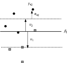
Individual and group residuals in a two-level model for the mean
Residuals at both levels are assumed to follow normal distributions with zero means: \(u_i\sim N(0,\sigma^2_u)\) and \(\varepsilon_{ij}\sim N(0,\sigma^2_e)\). All residuals are assumed at both levels are assumed to be independent. This partitions the variation in the between group variance, \(\sigma^2_u\), and the within group between individual variance, \(\sigma^2_e\). In this simple model, \(\sigma^2_u\) measure the between group difference, so to test whether there is a group difference in the populations, we need to test \(H_0:\;\sigma^2_u=0\) vs \(H_1:\;\sigma^2_u>0\). We can do this with a likelihood ratio test. The likelihood ratio test statistic is calculated as
\[LR=-2\log L_1-(-2\log L_2)\]
where \(L_1\) and \(L_2\) are the likelihood values from the null model and multilevel model above respectively. The log refers to natural logarithm. This test statistic will have a chi-square distribution with df = 1 since there is a difference of one parameter, \(\sigma^2_u\), between the two nested models. Rejection of the null hypothesis means that there are real group differences, so the mulitlevel model is preferred.
Example: Birth weights
Consider a study of birth weights. The data includes mothers from Georgia who have had 5 children. Is there significant variability in birth weights between mothers? In this example, we have a two level structure with the children nested within mothers.

Let’s fit the following model to this data:
\[BWEIGHT_{ij}=\beta_0+MOM_i+\varepsilon_{ij}\]
- \(BWEIGHT_{ij}=\text{ the birth weight of baby j from mom i}\)
- \(MOM_i\overset{iid}{\sim}N(0,\sigma^2_M)\)
- \(\varepsilon_{ij}\overset{iid}{\sim}N(0,\sigma^2_{e})\)
- The mom effects and residuals \(\varepsilon_{ij}\) are all independent.
We model the mother’s effect as random as we want to be able to generalize beyond the mothers in this study to the population of mothers. This also will allow us to account for the correlation of birth weights for infants from the same mother. If we look at a scatter matrix of the birth weights of child i vs child j from the same mother, it is clear that they are correlated.
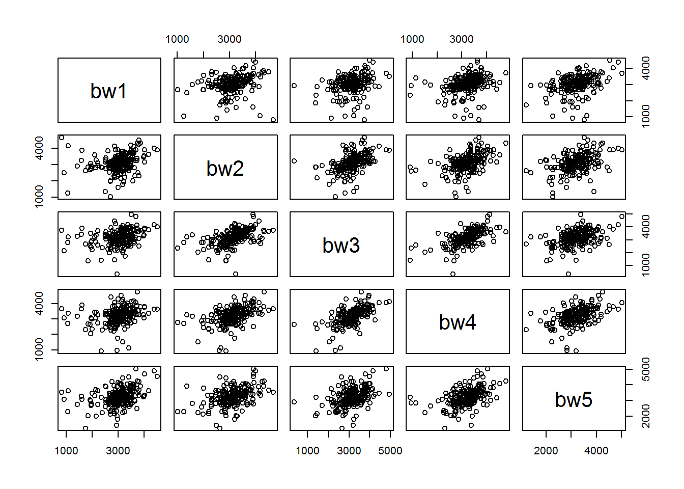
From looking at the scatterplot matrix, the birth weights between the infants from the same mother are indeed correlated and the correlation appears to be constant between all five infants. Fitting the multilevel model yields the follwing results.
## Linear mixed model fit by maximum likelihood  ['lmerMod']
## Formula: bweight ~ (1 | momid)
##    Data: gababies.dat
##
##      AIC      BIC   logLik deviance df.resid
##  15356.4  15371.1  -7675.2  15350.4      997
##
## Scaled residuals:
##     Min      1Q  Median      3Q     Max
## -5.4048 -0.4230  0.0325  0.5390  3.1643
##
## Random effects:
##  Groups   Name        Variance Std.Dev.
##  momid    (Intercept) 132976   364.7
##  Residual             203229   450.8
## Number of obs: 1000, groups:  momid, 200
##
## Fixed effects:
##             Estimate Std. Error t value
## (Intercept)  3135.46      29.46   106.4
## Data: gababies.dat
## Models:
## gababies.null: bweight ~ 1
## gababies.mod: bweight ~ (1 | momid)
## Df AIC BIC logLik deviance Chisq Chi Df Pr(>Chisq)
## gababies.null 2 15567 15577 -7781.7 15563
## gababies.mod 3 15356 15371 -7675.2 15350 212.99 1 < 2.2e-16 ***
## ---
## Signif. codes: 0 '***' 0.001 '**' 0.01 '*' 0.05 '.' 0.1 ' ' 1In this model, we have the following estimates:
- \(\hat{\beta_0}=3135.46\)
- \(\sigma^2_{M}=132976\)
- \(\sigma^2_e=203229\)
The intra-class correlation coefficient is
\[\dfrac{132976}{132976+203229}=0.396,\]
so 39.6% of the variability in birth weight is due to the variation in mothers. We can also interpret 0396 as the correlation between birth weights for two randomly selected babies from the same mother. The overall mean birth weight is estimated to be 3135.46 g. The log likelihood for the null model is \(\log L_1=-7781.7\) and the loglikelihood for the multilevel model is \(\log L_2=-7675.2\), so the likelihood ratio test statistic is
\[LR=-2\log L_1-(-2\log L_2)=-2(-7781.7)-(-2*-7675.2)=213\]
This results in a p-value of less than 0.0001 (\(<2.2e-16\)), so there is very strong evidence of between mother variability in birth weights.
Adding a Level 1 Variable
The simplest multilevel model with a single explanatory variable is
\[y_{ij}=\beta_0+\beta_1x_{ij}+u_i+\varepsilon_{ij}\].
In this model, the overall (cross-group) relationship between \(y\) and \(x\) is represented by a straight line with intercept \(\beta_0\) and slope \(\beta_1\). However, the intercept for a given group \(i\) is \(\beta_0+u_i\), i.e. it will be higher or lower than the overall \(\beta_0\) by an amount \(u_i\). The \(u_i\) is still assumed to be normal with mean 0 and variance \(\sigma^2_u\).
The model consists of two parts
- Fixed effects: \(\beta_0+\beta_1x_{ij}\)
- overall mean response for a given x
- Random effects: \(u_i+\varepsilon_{ij}\)
- random group effect and the individual random error.
This model allows the intercept of the regression line to vary between groups by modeling the group effect \(u_i\). To highlight the hierarchical structure, we can also write the model this way:
- Level 1: \(y_{ij}=\beta_{0i}+\beta_1x_{ij}+\varepsilon_{ij}\)
- Within a group, the mean response is modeled as a linear function of x where each group gets its own intercept.
- Level 2: \(\beta_{0i}=\beta_0+u_i\)
- Each group intercept is equal to an overall mean intercept for the population over all groups, \(\beta_0\), plut a group specfic random effect, \(u_i\), giving the unique group intercept.
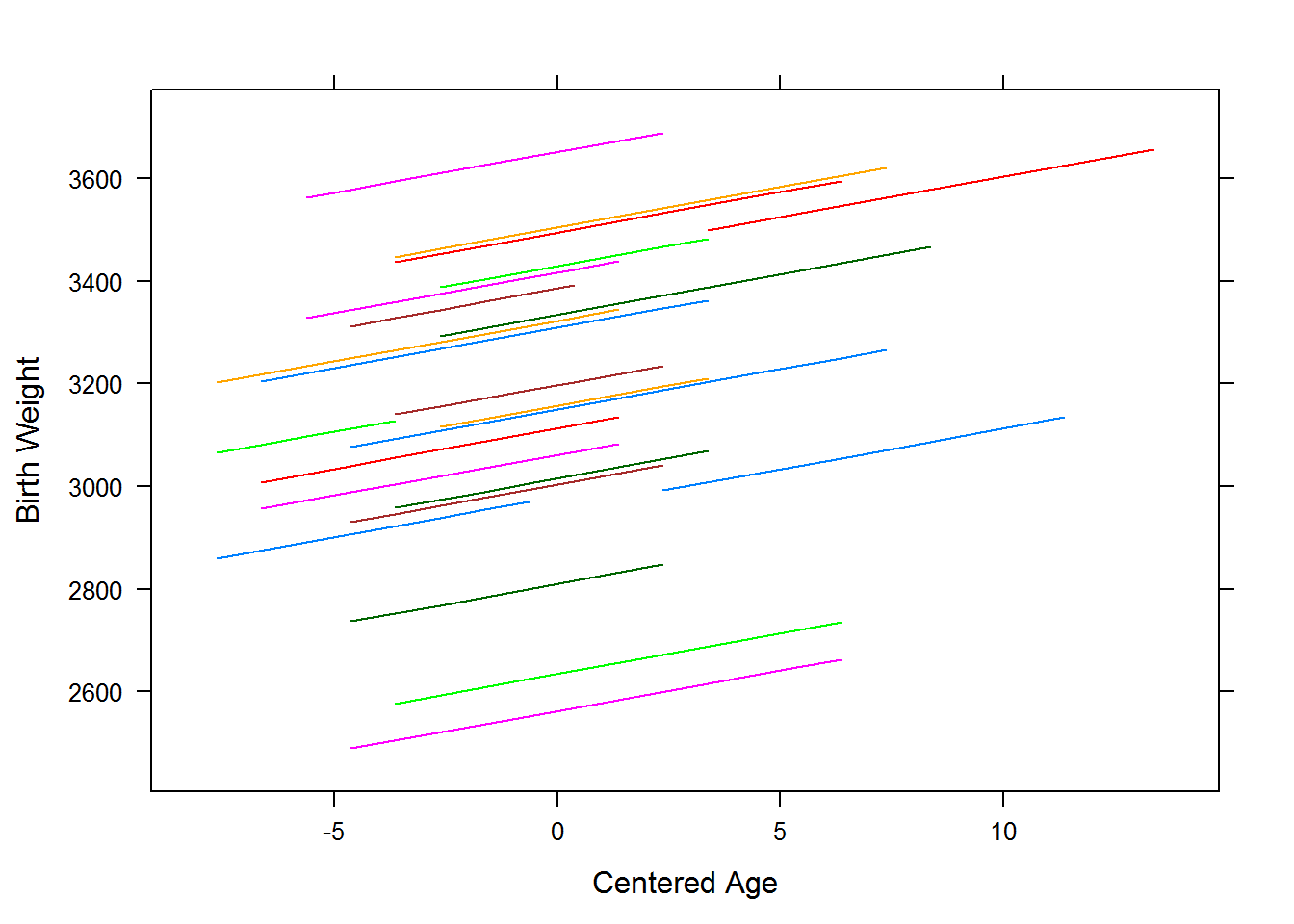
In this model, the intercept can vary from group to group, but the effect of the predictor x on the response is the same over all groups modeled by a constant slope \(\beta_1\). This means that the estimated regression equations for the groups will be parallel lines: \(\hat{y}_{ij}=\hat{\beta}_0 +\hat{\beta}_1x_{ij}+\hat{u}_i\). This is illustrated in the figure below.

Prediction lines from a random intercept model
Example: Birth weights
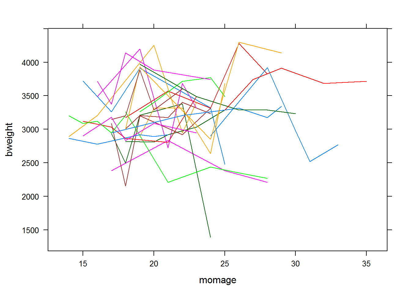
Let’s return the the birth weights example. Recall that this dataset contains measurements on infants for mothers in Georgia. Each mother in the dataset has had 5 children. The birth weight for each child is recorded in grams. In this example, we will also add the mother’s age during the birth of the child as a predictor for the birth weight. This is a level one variable since it changes with each birth.
The following shows a plot of the data for some of the individual moms.
The results for fitting the following model are given below:
\[BWEIGHT_{ij}=\beta_0+\beta_1*MOMAGE_{ij}+MOM_i+\varepsilon_{ij}\]
where,
- \(BWEIGHT_{ij}=\text{ the birth weight of baby j from mom i}\)
- \(MOMAGE_{ij}=\text{ age of mother i during birth of infant j}\)
- \(MOM_i\overset{iid}{\sim}N(0,\sigma^2_M)\)
- \(\varepsilon_{ij}\overset{iid}{\sim}N(0,\sigma^2_{e})\)
- The mom effects and residuals \(\varepsilon_{ij}\) are all independent.
## Linear mixed model fit by REML ['lmerMod']
## Formula: bweight ~ I(momage - mean(momage)) + (1 | momid)
##    Data: gababies.dat
##
## REML criterion at convergence: 15312
##
## Scaled residuals:
##     Min      1Q  Median      3Q     Max
## -5.1122 -0.4427  0.0469  0.5293  4.0901
##
## Random effects:
##  Groups   Name        Variance Std.Dev.
##  momid    (Intercept) 127796   357.5
##  Residual             199047   446.1
## Number of obs: 1000, groups:  momid, 200
##
## Fixed effects:
##                          Estimate Std. Error t value
## (Intercept)              3135.464     28.949   108.3
## I(momage - mean(momage))   15.799      3.099     5.1
##
## Correlation of Fixed Effects:
##             (Intr)
## I(-mn(mmg)) 0.000
## [1] 21.633The predicted regression equation for each of the individual moms shown above is:
The following table summarizes and compares the results of fitting the random intercept model with and with out the mom’s age at birth.
| Null Model |
Random Intercept with age |
|||
|---|---|---|---|---|
| Parameter | Estimate | Standard error |
Estimate | Standard error |
| β0 | 3135.46 | 29.46 | 3135.464 | 28.949 |
| β1 (centerd age) | - | - | 15.799 | 3.099 |
| σM2 | 132976 | - | 127796 | - |
| σe2 | 203229 | - | 199047 | - |
- For any mom, a 1 year increase in age is estimated to result in a 15.8 g increase in mean birth weight.
- The estimated average birth weight (over all groups) for a mother at mean age of 21.67 is 3135.5 grams.
- The 95% confidence interval for the mean mother’s intercept is \(3135.464\pm 1.96\sqrt{127796}=(2434.792,3836.136)\), so we are 95% confident that the mean birth weight for an infant of a mother at the mean age of 21.67 is between 2435 and 3836 grams.
- Note that the addition of age has lowered the level 1 variance, \(\sigma^2_e\), since it explains some of the variability in the responses.
- The between mother variance was also reduced. This indicates that the age distribution of the mother at the birth of each child varies between mothers.
- In particular, \(127796/(127796+199047)=39.1\%\) of the variation in birth weights is is explained by between mother differences, after accounting for age.
In general, adding a level one predictor will always reduce the level one variance, \(\sigma^2_e\). A level one predictor may increase, decrease or not affect the level 2 variance \(\sigma^2_M\). In order for the level 1 predictor to affect the level two variance, there must be some difference in the distribution of the level one predictor between the level 2 groups. To see how consider the following two situations: Throughout these two examples, we assume that there is a positive correlation between individual mother’s age at birth and birth weight, which is the same across all mother’s, and there is a mother effect on birth weight.
Scenario 1: Suppose that the mother’s mean of the age at birth of her 5 children, \(\bar{x}_i\), varies across mothers in such a way above average birth weights for the five children tend to have mother’s with high average age at birth over the five children. That is the average mother’s age is positively correlated with the average birth weight. At the individual level (i.e. for each mother), we find that the mother’s age is positively associated with the birth weight, that is mother’s who give birth later in life tend to have babies with a higher birth weight. In the model without the mother’s age as a predictor, all of the variablility is in the between mother variance, but since the association at the individual level and the mother (group) level is the same, adding the mother’s age as a predictor would explain some of this variability and decrease the between mother variance.
Scenario 2: Suppose that the mother’s mean of the age at birth of her 5 children, \(\bar{x}_i\), varies across mothers in such a way above average birth weights for the five children tend to have mother’s with below average age at birth over the five children. That is the average mother’s age is negatively correlated with the average birth weight. At the individual level (i.e. for each mother), we find that the mother’s age is positively associated with the birth weight, that is mother’s who give birth later in life tend to have babies with a higher birth weight. In the model without the mother’s age as a predictor, all of the variablility is in the between mother variance, but since the association at the individual level and the mother (group) level is the different, adding the mother’s age as a predictor would cause the between mother variance to increase. In this case, mother effect’s look weaker if we do not account for the mother’s age. Adding mother’s age to the model will reveal stronger mother effects, leading to the increase in the between mother variance.