Lab 3: Linear Mixed Models in R
The following Nepali dataset is from a public health study of growth in Nepali children. Vitamin A is an essential vitamin for growth, and it is known to be important in growth for vitamin A deficient children. In this study, all children were provided vitamin A and their weight was measured every four months for up to 5 follow-up visits. In this lab, we will consider the following variable:
- \(y_{ij}=\text{ child i's weight in kilograms at visit j}\)
- \(x_{1ij}=\text{ child's age in months}\)
- $x_{2i}=
First, let’s do some exploratory data analysis by looking at some “spaghetti” plots.
library(faraway)##
## Attaching package: 'faraway'## The following object is masked from 'package:lattice':
##
## melanomalibrary(lattice)
nep.dat <- nepali
nep.dat$sex <- factor(nep.dat$sex,levels=c(1,2),labels=c("male","female"))
nep.dat$ageGM <- rep(tapply(nep.dat$age,nep.dat$id,mean),each=5)
xyplot(wt~age|sex,groups=id,data=nep.dat,type="l")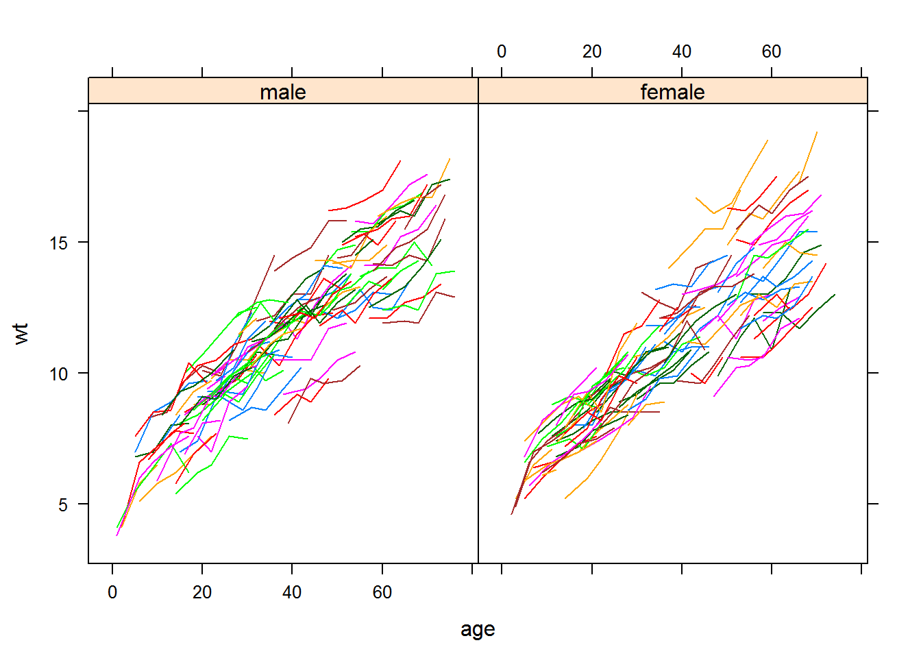
We will consider a random intercept model with age and gender as covariates, since it seems that the growth pattern is roughly linear for each child. The slopes for age do not seem to vary from subject to subject, but there is variability in the intercepts between the genders and this variability changes with age.
library(lme4)
nep.mod1 <- lmer(wt~sex+I(age-ageGM)+ageGM+(1+sex|id),data=nep.dat,REML=FALSE)
summary(nep.mod1)
## Linear mixed model fit by maximum likelihood ['lmerMod']
## Formula: wt ~ sex + I(age - ageGM) + ageGM + (1 + sex | id)
## Data: nep.dat
##
## AIC BIC logLik deviance df.resid
## 1783.8 1822.0 -883.9 1767.8 869
##
## Scaled residuals:
## Min 1Q Median 3Q Max
## -3.5068 -0.4859 0.0006 0.5233 4.2660
##
## Random effects:
## Groups Name Variance Std.Dev. Corr
## id (Intercept) 1.679995 1.29615
## sexfemale 0.009835 0.09917 1.00
## Residual 0.190381 0.43633
## Number of obs: 877, groups: id, 197
##
## Fixed effects:
## Estimate Std. Error t value
## (Intercept) 5.844754 0.246281 23.73
## sexfemale -0.343497 0.195251 -1.76
## I(age - ageGM) 0.132921 0.002707 49.11
## ageGM 0.144419 0.005471 26.40
##
## Correlation of Fixed Effects:
## (Intr) sexfml I(-aGM
## sexfemale -0.379
## I(ag-ageGM) 0.007 -0.003
## ageGM -0.852 0.039 -0.001VarCorr(nep.mod1)$id## (Intercept) sexfemale
## (Intercept) 1.6799947 0.128542236
## sexfemale 0.1285422 0.009835214
## attr(,"stddev")
## (Intercept) sexfemale
## 1.29614608 0.09917265
## attr(,"correlation")
## (Intercept) sexfemale
## (Intercept) 1 1
## sexfemale 1 1Next, let’s see the prediction lines for this fitted model.
xyplot(predict(nep.mod1)~age|sex,groups=id,data=na.omit(nep.dat),type="l")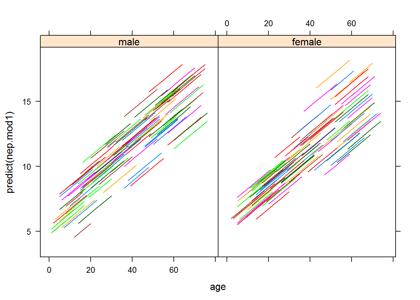
The gender effect term does not appear to be significant. The following performs a likelihood ratio test of this term. To do this test, we need to fit the two nested models to test for the significance of the random slope term.
nep.mod2 <- lmer(wt~I(age-ageGM)+age+(1+I(age-ageGM)|id),data=nep.dat,REML=FALSE)
anova(nep.mod1,nep.mod2)
## Data: nep.dat
## Models:
## nep.mod2: wt ~ I(age - ageGM) + age + (1 + I(age - ageGM) | id)
## nep.mod1: wt ~ sex + I(age - ageGM) + ageGM + (1 + sex | id)
## Df AIC BIC logLik deviance Chisq Chi Df Pr(>Chisq)
## nep.mod2 7 1713.7 1747.1 -849.83 1699.7
## nep.mod1 8 1783.8 1822.0 -883.89 1767.8 0 1 1In this case, there is no evidence of a gender effect. Let’s see what fit and the prediction lines look like for the reduced model.
summary(nep.mod2)## Linear mixed model fit by maximum likelihood ['lmerMod']
## Formula: wt ~ I(age - ageGM) + age + (1 + I(age - ageGM) | id)
## Data: nep.dat
##
## AIC BIC logLik deviance df.resid
## 1713.7 1747.1 -849.8 1699.7 870
##
## Scaled residuals:
## Min 1Q Median 3Q Max
## -3.2130 -0.4233 0.0252 0.4839 2.4431
##
## Random effects:
## Groups Name Variance Std.Dev. Corr
## id (Intercept) 1.863350 1.3650
## I(age - ageGM) 0.001529 0.0391 0.28
## Residual 0.134204 0.3663
## Number of obs: 877, groups: id, 197
##
## Fixed effects:
## Estimate Std. Error t value
## (Intercept) 5.436779 0.226145 24.041
## I(age - ageGM) -0.017801 0.006535 -2.724
## age 0.150867 0.005405 27.914
##
## Correlation of Fixed Effects:
## (Intr) I(-aGM
## I(ag-ageGM) 0.798
## age -0.901 -0.825xyplot(predict(nep.mod2)~age|sex,groups=id,data=na.omit(nep.dat),type="l")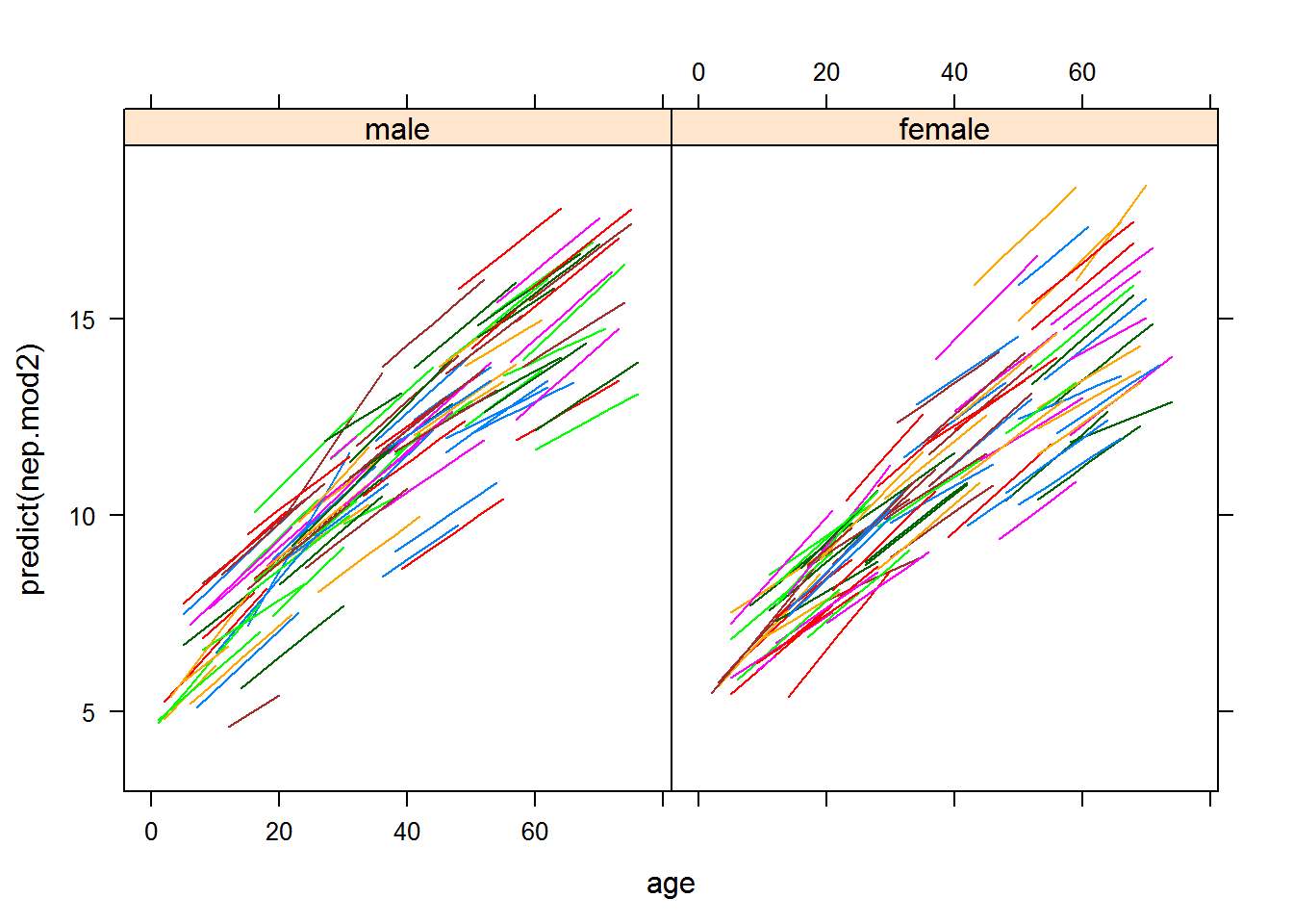 We can futher test to see if the gender effect is significant.
nep.mod3 <- lmer(wt~age+(1|id),data=nep.dat,REML=FALSE)
anova(nep.mod2,nep.mod3)
## Data: nep.dat
## Models:
## nep.mod3: wt ~ age + (1 | id)
## nep.mod2: wt ~ I(age - ageGM) + age + (1 + I(age - ageGM) | id)
## Df AIC BIC logLik deviance Chisq Chi Df Pr(>Chisq)
## nep.mod3 4 1782.9 1802.0 -887.46 1774.9
## nep.mod2 7 1713.7 1747.1 -849.83 1699.7 75.26 3 3.187e-16 ***
## ---
## Signif. codes: 0 '***' 0.001 '**' 0.01 '*' 0.05 '.' 0.1 ' ' 1