Why Should We Consider Multilevel Models?

What can go wrong?

Let’s consider a simple example. Lack of digestive enzymes in the intestine can cause bowel absorption problems. This will be indicated by excess fat in the feces. Pancreatic enzyme supplements can be given to ameliorate the problem. The data in the table below come from a study to determine if there are differences due to the form of the supplement: a placebo (none), a tablet, an uncoated capsule (capsule), and a coated capsule (coated).

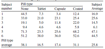
We can think of this as a repeated measures dataset, since each cat does all four treatements at some point (this is called a cross-over design). We also saw earlier, that this can be pictured as a hierarchical dataset of obeservations nested within patient. The only predictor is the pill type: placebo, tablet, uncoated capsule, and coated capsule (which is a level 1 variable). First, let’s ignore the clustering. Since we have a quantitative response and a single categorical predictor, we could use a one-way ANOVA to anlyze this data. Recall that the one-way ANOVA assumes,

• all observations are independent
• constant variance between groups
• normal responses.

This results in the following model:

\[\text{FECCAT}_{ij}=\mu +\text{PillType}_j+\varepsilon_{ij}\]

where the residuals, \(\varepsilon_{ij}\), are assumed to be independent and have a normal distribution with mean zero and variance \(\sigma^2_\varepsilon\). Below is the analysis of the data using one-way ANOVA.Here \(FECCAT_{ij}\) represents the fecal fat measurement for cat \(i\) on pill type \(j\).

## 
## Call:
## lm(formula = fecfat ~ ptype, data = feccat.dat)
## 
## Residuals:
##     Min      1Q  Median      3Q     Max 
## -28.683 -12.154  -5.350   9.417  37.133 
## 
## Coefficients:
##             Estimate Std. Error t value Pr(>|t|)  
## (Intercept)  17.4167     7.7424   2.250   0.0359 *
## ptypeCoated  13.6500    10.9494   1.247   0.2269  
## ptypeNone    20.6667    10.9494   1.887   0.0737 .
## ptypeTablet  -0.8833    10.9494  -0.081   0.9365  
## ---
## Signif. codes:  0 '***' 0.001 '**' 0.01 '*' 0.05 '.' 0.1 ' ' 1
## 
## Residual standard error: 18.96 on 20 degrees of freedom
## Multiple R-squared:  0.2183, Adjusted R-squared:  0.101 
## F-statistic: 1.862 on 3 and 20 DF,  p-value: 0.1687

Notice that the overall ANOVA F test has a p-value of 0.1687. Based on the one-way ANOVA, we would conclude that there is no effect of pill type.

It is important to note that we have made a grave mistake here. We have ignored the correlation between the observations made on the same cat. This violates the independence assumption of ANOVA. So, how do we take into account this correlation structure? One way is with a linear mixed model. The following model is an example of a random intercept model that takes in to account the between subject variation. We would expect some cats to have naturally higher fat amounts in their fecal matter than others. To accomodate this, we include a random subject effect in the model:

\[FECCAT_{ij}=\mu +SUBJECT_i+PILLTYPE_j+\varepsilon_{ij}\]

where the residuals, \(\varepsilon_{ij}\), are assumed to be independent and have a normal distribution with mean zero and variance \(\sigma^2_\varepsilon\), the subject effects are a random sample from a normal distribution with mean 0 and variance \(\sigma^2_{subj}\) and the all the errors are independent of all the subject effects.This serves two purposes:

• First, it captures the idea that the subjects in our experiment are assumed to be a random sample from a larger population of subjects to which we wish to draw inferences. Otherwise, the conclusions from our experiment would be scientifically uninteresting, as they would apply only to a select group of six subjects.
• Second, as we will examine in detail in the next section, the inclusion of a subject effect (along with an assigned distribution) models a correlation in the outcomes.

Below is the analysis using the random effects model.

## Linear mixed model fit by REML ['lmerMod']
## Formula: fecfat ~ (1 | subject) + ptype
##    Data: feccat.dat
## 
## REML criterion at convergence: 169.1
## 
## Scaled residuals: 
##      Min       1Q   Median       3Q      Max 
## -1.21005 -0.61507 -0.00273  0.45711  1.72562 
## 
## Random effects:
##  Groups   Name        Variance Std.Dev.
##  subject  (Intercept) 252.7    15.90   
##  Residual             107.0    10.34   
## Number of obs: 24, groups:  subject, 6
## 
## Fixed effects:
##             Estimate Std. Error t value
## (Intercept)  17.4167     7.7424   2.250
## ptypeCoated  13.6500     5.9721   2.286
## ptypeNone    20.6667     5.9721   3.461
## ptypeTablet  -0.8833     5.9721  -0.148
## 
## Correlation of Fixed Effects:
##             (Intr) ptypCt ptypNn
## ptypeCoated -0.386              
## ptypeNone   -0.386  0.500       
## ptypeTablet -0.386  0.500  0.500

## Analysis of Variance Table
##       Df Sum Sq Mean Sq F value
## ptype  3 2008.6  669.53  6.2574

## [1] 0.005731083

Now that we have taken into account the correlation, the p-value for testing for a pill type effect is 0.0057, which is highly significant. This means that excluding the dependence structure inflated the p-value.

In general, ignoring the dependence structure will lead to incorrect standard errors, which leades

• incorrect p-values - these can be inflated as in the previous example or made to be too small
• incorrect confidence intervals - the incorrect standard errors can lead to confidence intervals that are too wide or narrow.

The idea behind why this happens has to do with the amount of independent data that you have known as the effective sample size. Consider a two-level structure with 5000 individuals organised in 100 groups. For simplicity suppose that each group contains 50 individuals. In a single-level model standard errors are calculated on the assumption that the individuals in the sample provide 5000 independent pieces of information. When outcomes are clustered, however, there will be fewer than 5000 independent observations. The number of independent observations is called the effective sample size (ESS) and depends on the degree of clustering (as measured by the intra-class correlation or variance partition coefficient). For example, consider the extreme situation where the intra-class correlation (see below) is 1 (all individuals in a group have the same y value) and therefore each group provides only one independent observation. In that case the ESS would be equal to the number of groups, i.e.,100 rather than 5000, and standard errors from a multilevel analysis would therefore be substantially higher than those from a single-level analysis. Underestimation in a single-level model is especially severe for coefficients of variables that are defined at the group level.