Random Slope Models

The random intercept model assumes the relationship between $y$ and $x$ is the same in each group, i.e. that the slope $\beta_1$ is fixed across groups. We can relax this constraint by allowing the slopes to vary randomly across groups, leading to the random slope model:

\[y_{ij}=\beta_0+\beta_1x_{ij}+u_{0i}+u_{1i}x_{ij}+\varepsilon_{ij}\]

which can be written in the hierarchical form:

Level 1: $y_{ij}=\beta_{0i}+\beta_{0j}x_{ij}+\varepsilon_{ij}$
Level 2 (intercept): $\beta_{0i}=\beta_0+u_{0i}$
Level 2 (slope): $\beta_{1i}=\beta_1+u_{1i}$

In this model, the overall relationship of the mean response, across groups, is modeled as $\beta_0+\beta_1x_{ij}$. The subject specific relationship of y and x is modeled as $y_{ij}=(\beta_0+u_{0i})+(\beta_1+u_{1i})x_{ij}+\varepsilon_{ij}$. Now, with the addition of a new term, $u_{1i}x_{ij}$, to the model, the slopes can vary between groups. In this model,

$u_{0i}$ and $u_{1i}$ are assumed to jointly follow a normal distribution with means 0 and
- $\text{Var}(u_{0i})=\sigma^2_{u0}$
- $\text{Var}(u_{1i})=\sigma^2_{u1}$
- $\text{Cov}(u_{0i},u_{1i})=\sigma_{u01}$

What do these parameters mean?

The variance of $u_{0i}$, $\sigma^2_{u0}$, describes the variation in the intercept terms between groups, $\beta_0+u_{0i}$, with $\beta_0$ as the overall mean intercept between all groups
The variance of $u_{1i}$, $\sigma^2_{u1}$, describes the variation in the slope terms between groups, $\beta_1+u_{1i}$, with $\beta_1$ as the overall mean slope between all groups.
The covariance between $u_{0i}$ and $u_{1i$}, describes the relationship between the slope and intercept terms. A positive covariance means that groups with higher y intercept terms tend to have higher slope terms. This will lead to a fanning out of subject specific regression lines when plotted. Similary, a negative covariance means that groups with higher y-intercept terms then to have lower slope terms. This will lead to a fanning in of regression lines when plotted. The interpretation is similar to correlations.

The term $u_{1i}x_{ij}$ can be though of as an interaction term between the groups and the predictor, e.g. between the mothers age and the mom effect.

The figure below illustrates the prediction lines obtained from a random slope model.The intercepts of the group lines are the same as before in the random intercept model, but the slope is no longer the same for each group. The slope of the line for group 1 is steeper than the slope for the average line by an amount $\hat{u}_{11}$, while group 2 has a slope which is smaller by an amount $_{12}. For these two groups, a high intercept is associated with a steep slope. If this pattern holds when all groups are considered, the intercept-slope covariance will be positive and the group lines will fan out.

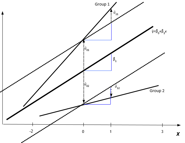
Prediction lines from a random slope model

Interpretation of different slope

Suppose that the figure above shows the prediction lines for the relationship between blood glucose levels (y) and body mass index (x). Across the range of x, cluster one has a higher blood glucose level, and the difference between the two groups widens as body mass index increases. Thus the effect of body mass index on blood glucose levels is more severe in cluster 1 than it is in cluster 2. It would be much more important for patients in cluster 1 to lower their BMI than for patients in cluster 2. In cluster 2, since the line is flatter, there is not as much of a difference in blood glucose levels for those with high or low body mass index.

Another example where the relative slopes of the prediction lines measures equity is in the relationship between health and income for different areas. Areas with large income inequalities in health will tend to have steep slopes, while areas with less inequality, perhaps as a result of efforts to improve access to health care among low income households, will tend to have shallower slopes.

Example of random slope: Allowing the relationship between birth weight and mom’s age at infants birth to vary from mother to mother

Let’s return to the birth weight example, but now we will include a random slope for the centered mothers age. The random slope model is:

\[BWEIGHT_{ij}=\beta_0+\beta_1*MOMAGEC_{ij}+MOM_{i0}+MOM_{i1}*MOMAGEC_{ij}+\varepsilon_{ij}\] where

$MOM_{i0}$ and $MOM_{i1}$ are i.i.d. jointly normal with mean 0, $\text{Var}(MOM_{i0})=\sigma^2_{M0}$, $\text{Var}(MOM_{i1})=\sigma^2_{M1}$, and $\text{Cov}(MOM_{i0},MOM_{i1})=\sigma_{M01}$.
The error terms, $\varepsilon_{ij}$, are i.i.d. with a normal distribution with mean 0 and variance $\sigma^2_e$.

## Linear mixed model fit by maximum likelihood  ['lmerMod']
## Formula: bweight ~ momageC + (1 + momageC | momid)
##    Data: gababies.dat
## 
##      AIC      BIC   logLik deviance df.resid 
##  15329.6  15359.1  -7658.8  15317.6      994 
## 
## Scaled residuals: 
##     Min      1Q  Median      3Q     Max 
## -4.9962 -0.4302  0.0466  0.5325  3.9964 
## 
## Random effects:
##  Groups   Name        Variance Std.Dev. Corr
##  momid    (Intercept) 125758.4 354.62       
##           momageC        130.2  11.41   0.78
##  Residual             196652.7 443.46       
## Number of obs: 1000, groups:  momid, 200
## 
## Fixed effects:
##             Estimate Std. Error t value
## (Intercept) 3136.227     28.841  108.74
## momageC       21.039      3.994    5.27
## 
## Correlation of Fixed Effects:
##         (Intr)
## momageC 0.187

## [1] ""

## [1] "Variance Covariance Matrix of Random Effects"

##             (Intercept)   momageC
## (Intercept)  125758.424 3158.5276
## momageC        3158.528  130.1851
## attr(,"stddev")
## (Intercept)     momageC 
##   354.62434    11.40987 
## attr(,"correlation")
##             (Intercept)   momageC
## (Intercept)   1.0000000 0.7806125
## momageC       0.7806125 1.0000000

The following table summarizes the difference in the parameters between the random intercept model and the random slope model.

	Random Intercept		Random Slope
Parameter	Estimate	SE	Estimate	SE
β₀	3135.464	28.949	3136.227	28.84
β₁ (centered at mean age)	15.799	3.099	21.04	3.99
Mom level random part
σ_M0²	127796	-	125758.4	-
σ_M1²	-	-	130.2	-
σ_M01	-	-	3158.53	-
Individual level random part
σ_e²	199047	-	196653	-

The grand mean y-intercept term, $\beta_0$, tells us that the mean birth weight of infants across all mom’s at the average age of 21.6 is 3136.227 grams
The grand mean slope term, $\beta_1$, tells us that the mean birth weight of infants born to moms at the mean age of 21.6 across all moms is estimated to increase by 21.04 grams for each one year increase in the mother’s age at birth.

The random slope model has two additional terms: the between mom variance in the slopes, $\sigma^2_{M1}$, and the covariance between the mom intercepts and the mom slopes, $\sigma_{M01}$. The likelihood ratio test contrasting the random slope model with the random intercept model is given below.

## Data: gababies.dat
## Models:
## gababies.mod2: bweight ~ momageC + (1 | momid)
## gababies.mod3: bweight ~ momageC + (1 + momageC | momid)
##               Df   AIC   BIC  logLik deviance Chisq Chi Df Pr(>Chisq)  
## gababies.mod2  4 15333 15352 -7662.3    15325                          
## gababies.mod3  6 15330 15359 -7658.8    15318 7.039      2    0.02961 *
## ---
## Signif. codes:  0 '***' 0.001 '**' 0.01 '*' 0.05 '.' 0.1 ' ' 1

The p-value is 0.02961 indicating that there is strong evidence that the effect of the mother’s age at birth on birth weight varies across mom’s.

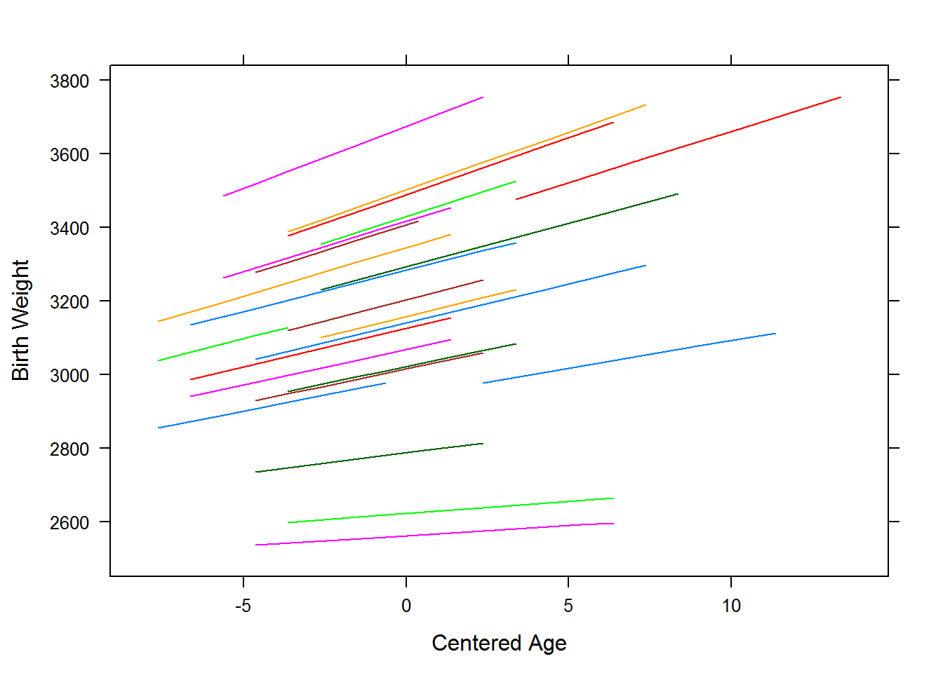
The figure above shows the mom prediction lines for birth weight by age obtained from the random slope model. All mom’s have a positive slope, so across all moms it is the first child that tends to have the lowest birth weight. The positive covariance between the the slopes and intercepts implies that mom’s with a large intercept (high mean birth weight at mean age, i.e. $\MOM_{0i}>0$) tend to have larger slopes (stronger positive relationship between mother’s age at birth and birth weight). The correlation betwen the intercepts and slopes of the mom regression lines is

\[\rho_{M01}=\dfrac{3158.53}{\sqrt{125758*130}}=0.78.\]

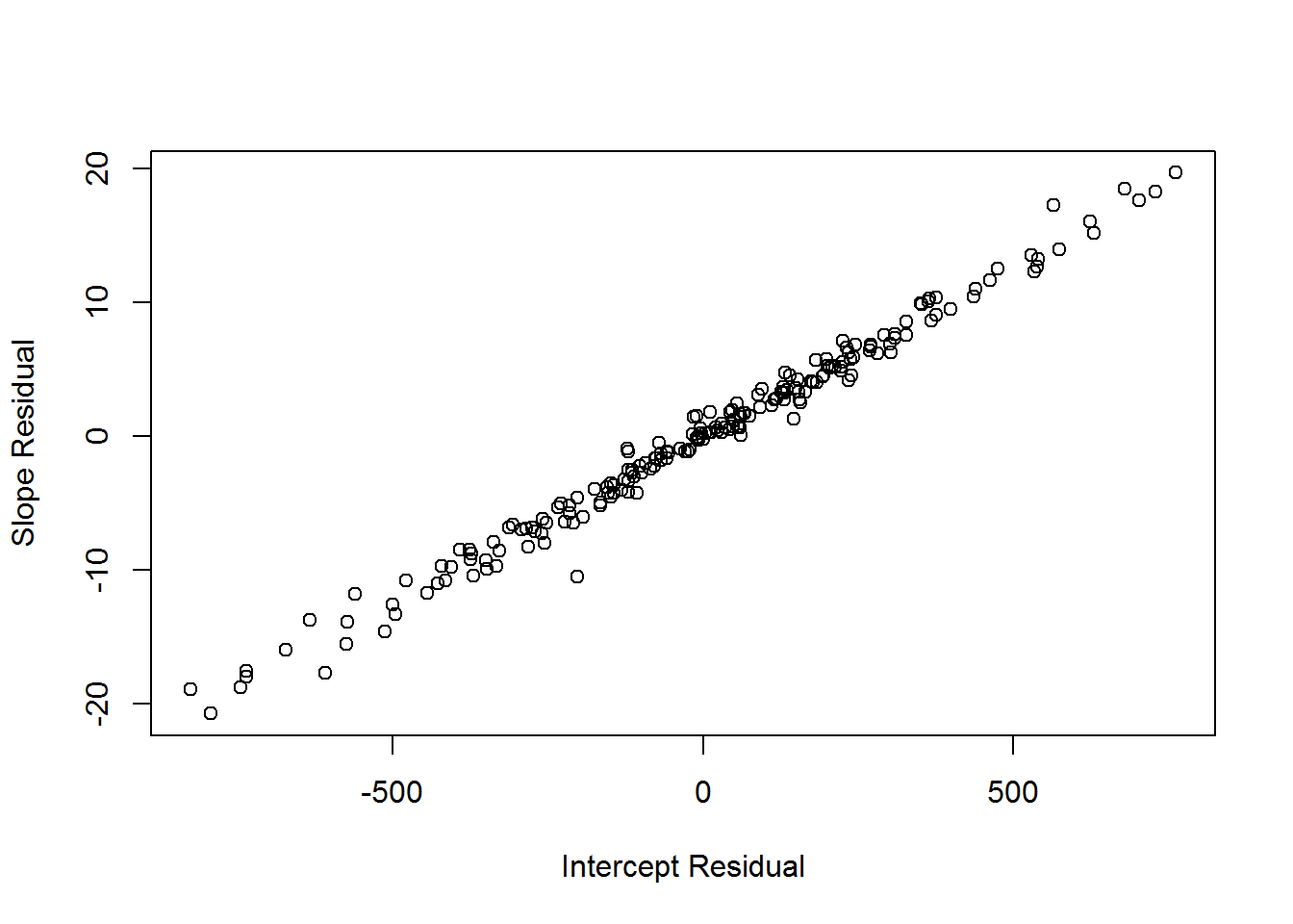
Each point represents a mother. The x coordinate is the mom’s random intercept effect, $MOM_{0i}$ and the y coordinate is the mother’s random slope effect, $MOM_{1i}$.

Between group variance

In the random intercept model, the between group variance is constant, i.e. it does not depend on the value of a predictor. In the random intercept model, the variation between groups is modeled by the subject specific random effects that appear in the model as: $u_{0i}+u_{1i}x_{ij}$. It can be shown that the variance of this term is

\[\begin{align*}\text{Var}(u_{0i}+u_{1i}x_{ij}) &=\text{Var}(u_{0i})+2x_{ij}\text{Cov}(u_{0i},u_{1i})+\text{Var}(u_{1i})\\ &= \sigma^2_{u0}+2x_{ij}\sigma_{i01}+\sigma^2_{u1}x_{ij}^2\end{align*}\]

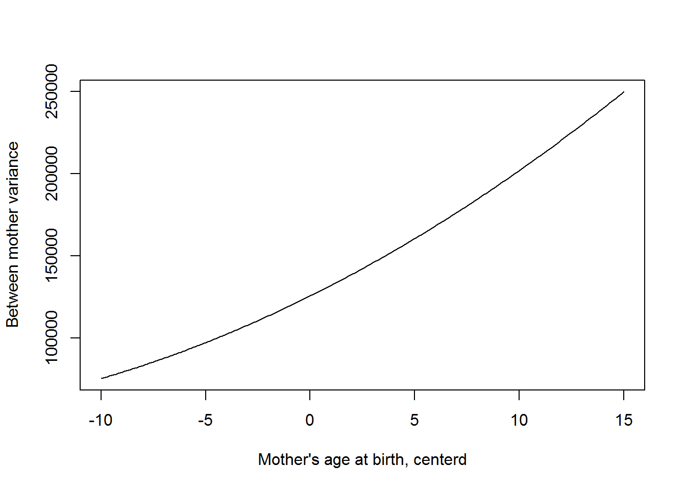
which is a quadratic function in x. Fromt he output about, the estimated between group variance at $x_{ij}$ is

\[\text{Between mom variance} = 125758+2*3159*x_{ij}+130x_{ij}^2=125758+6318*x_{ij}+130x_{ij}^2.\]

This function is plotted below. Between mom differences in birth weight are greater mom’s giving birth after the mean age (i.e among older mothers).

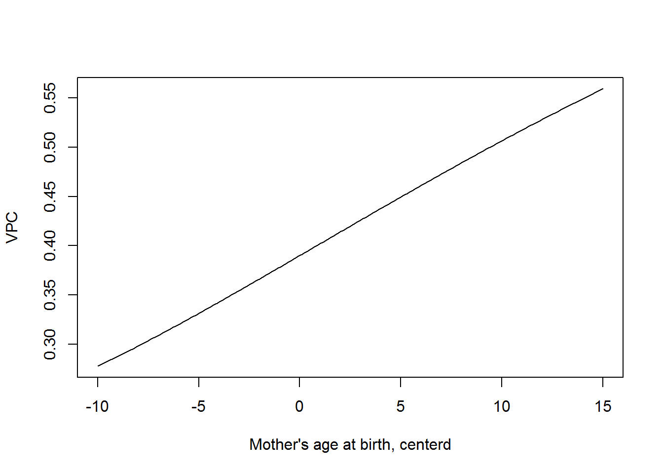
Now that we have a predictor, we can calculate the variance partition coefficent. With out a predictor this is just the intra-class correlation we saw earlier. The VPC is the percent of the variation in the response due to between group differences. In this case is given by

\[VPC=\dfrac{125758+6318*x_{ij}+130x_{ij}^2}{(125758+6318*x_{ij}+130x_{ij}^2)+196693}\].

The percentage of the variation in birth weights due to between mom difference also increases with mothers age at birth.